Excel dynamic ranges
Microsoft Excel has many Visual Basic for Application (VBA) features that are seemingly not well understood. One of these features is passing a range value into a VBA procedure (a Sub) or function. The following example demonstrates how to pass a dynamic range to a local multiple dimensional array, and process the uploaded data in a VBA function.
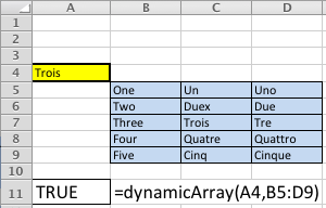
My sample spreadsheet looks like the screen shot below. The formula call is in cell A11 and the text of the formula is in cell B11.
I left a debug MsgBox() call that demonstrates how you size a range. This shows the range above based on zero-based numbering, which means 5 rows are reported as 4 rows because 0 contains a row, and 3 columns are reported as 2 columns for the same reason. If the dialog looks strange to a Windows user, that’s because it’s one generated on a Mac OS X running Excel 2011. 🙂
I kept this as simple as possible to demonstrate the how to do this. Unfortunately, feedback required adding more extensive comments and making it a bit more bulletproof on concepts. The variable names were chosen to help read the syntax. Two loops are used to demonstrate (a) how you assign the range values to a multidimensional array, and (b) how you read the array values in your VBA code.
1 2 3 4 5 6 7 8 9 10 11 12 13 14 15 16 17 18 19 20 21 22 23 24 25 26 27 28 29 30 31 32 33 34 35 36 37 38 39 40 41 42 43 44 45 46 47 48 49 50 51 52 53 54 55 56 57 58 59 60 61 62 | Function dynamicArray(lookupValue As String, table As Range) ' Define the row starting cell, Row n maps to the first row where the range is found in the spreadsheet. ' Row 1 is the first row and 1,048,576 is the last possible row. Dim rowStart As Integer Dim rowSize As Integer ' Define the column starting cell, Column A maps to 1, Column B maps to 2, et cetera. ' Column A is the first column and XFD is the last possible column. Dim columnStart As Integer Dim columnSize As Integer ' Create a dynamic multiple dimension array without any physical size. Dim multidimensionArray As Variant ' Define and declare a local returnValue variable. Dim returnValue As Boolean returnValue = False ' Assign the starting row and column values, and the length of values. ' Since you need to add the row and column to the starting grid coordinates, you need to use 0-based numbering, ' which means you subtract one from the length. rowStart = table.Row rowSize = table.Rows.Count - 1 columnStart = table.Column columnSize = table.Columns.Count - 1 ' This demonstrates that the range starts in the row and column, and ' the length and width of the multiple dimension array. ' ---------------------------------------------------------------------- ' Insert single quotes for the next two lines to suppress testing the program with variables. MsgBox ("(RowStart [" + CStr(rowStart) + "], (ColStart [" + CStr(columnStart) + "]) " + _ "(RowSize [" + CStr(rowSize) + "] ColSize [" + CStr(columnSize) + "])") ' ---------------------------------------------------------------------- ' Redimension the arrays maximum size, rows first, columns second. ReDim multidimensionArray(rowSize, columnSize) ' Read through the range and assign it to a local and dynamically sized array variable. ' An important note to those unfamilar with the Cells function, it works on the active worksheet and uses two ' parameters, the absolute row and column number or relative row and column numbers. In this sample, the ' easiest solution is to use absolute row an dolumn numbers. For i = 0 To rowSize For j = 0 To columnSize multidimensionArray(i, j) = CStr(Cells(rowStart + i, columnStart + j)) Next j Next i ' Read through the local variable range and view the content set. For i = 0 To rowSize For j = 0 To columnSize ' Check if the lookupValue has been found and return true. If lookupValue = CStr(multidimensionArray(i, j)) Then returnValue = True Exit For End If Next j Next i ' Return a Boolean value: true when found and false when not found. dynamicArray = returnValue End Function |
You would call it with syntax like that below. The range can be any valid range value in Excel, which is any two cell references separated by a colon.
=dynamicArray("LookupString",A1:G5) |
As always, I hope this helps others looking for a way to perform this task natively in Microsoft Excel. As an addendum, I thought the absence of a code example for VB on the MSDN web page was quite interesting.

