Archive for the ‘Excel 2008’ Category
Excel string parsing
Parsing strings isn’t the easiest thing to do in Excel 2007 or Excel 2008 but it is an important thing to know how to do. You’ll learn how to parse a set names into first, middle and last names. You can find the data set for these examples at the bottom of the blog post.
Parsing the left substring ↓
This shows you how to parse a left substring from a text cell in Microsoft Excel.
There are two built in functions that let you parse dynamic substrings from the left of a string. They are the LEFT and FIND functions. The LEFT function actually does the parsing but the FIND function lets you dynamically find a delimiting character, like a space.
Assuming cell A1 holds the value of Joseph F. Smith, you can parse Joseph by using a static value of seven for the first white space in the string. This works because each character maps to a string, and strings start with the number one. The LEFT function supports three formal parameters, the first is the string you’re parsing, the second is where to stop, and the third is where to start. The position you start at is assumed to be one, which makes the last parameter an optional parameter. You only provide the start with parameter when you want to start someplace other than the left most position.
This is the simplest use of the LEFT function with its two required parameters.
=LEFT(A1,7) |
It returns the substring Joseph from the string Joseph F. Smith, which is stored in cell A1.
The simplest solution merely illustrates a concept. You’re not going to do this unless you have a bit more data. Naturally, the list of first names have different lengths in the real world. You must include the FIND function inside the call to the LEFT function to make your function dynamic. The FIND function lets you capture the position of a white space delimiter.
The FIND function supports three formal parameters, the first is the substring you’re looking for in the string, the second is the string to search, and the third is where to start. Like the LEFT function, the position you start at is assumed to be one, which makes the last parameter an optional parameter. You only provide the start with parameter when you want to start someplace other than the left most position. While not required, you should consider always providing the start with parameter to the FIND function.
The following shows you how to use the FIND function to locate the first occurrence of a white space in a string stored in cell A1.
=FIND(" ",A1,1) |
You can now make you’re LEFT function dynamic by putting the FIND function inside it. As qualified, the FIND function looks for the first occurrence of a white space, and returns it into the second parameter of the LEFT function. The sample formula now has a nested function, which makes it a mega formula in Microsoft Excel parlance. The following sample also includes the optional start with parameter for clarity.
=LEFT(A1,FIND(" ",A1,1),1) |
The problem with the foregoing solution occurs when a name in the list doesn’t have a middle initial or name, or last name. The lack of a second name means that there won’t be any white space between to substrings in the base string. This situation causes the logic to fail because the FIND function returns a #VALUE! error when it can’t find a white space in the string.
You can prevent the error by wrapping the nested FIND function and LEFT function inside two IFERROR functions. This IFERROR function returns the positional value of the FIND function, or an alternative copy of the base string.
=IFERROR(FIND(" ",A1,1),A1) |
This type of logic inside the LEFT function causes the LEFT function to fail when the base string is returned to it instead of a position number. You must wrap the LEFT function inside another IFERROR function to guarantee that you don’t throw an error. This also lets you return the base string as the valid substring when appropriate.
=IFERROR(LEFT(A1,IFERROR(FIND(" ",A1),A1)-1),A1) |
Assuming you put this formula in cell C1, you could copy this relative reference formula down in a column. It would require that you had a list of full names that followed a first name, white space, middle initial or name, white space, and last name in the A column.
Parsing the right substring ↓
This shows you how to parse a right substring from a text cell in Microsoft Excel.
There are three built in functions that let you parse dynamic substrings from the right of strings. They are the RIGHT and FIND functions that you may have covered when reading how to parse from the left. The LEN function is the other function, and it lets you find the length of a string. Together these functions lets you find the length of a substring on the right.
The RIGHT function actually does the parsing but the FIND and LEN functions let you dynamically find where to cut a substring out of a base string. This example continues to use the string Joseph F. Smith.
The RIGHT function has only two required parameters. The first parameter is the string that you’re parsing. The second parameter is the length of the substring. If you inspect the string, Smith is only five characters long. A static call to the RIGHT function is shown below.
=RIGHT(A1,5) |
It returns the substring Smith from the string Joseph F. Smith, which is stored in cell A1.
Like the LEFT function example, this static approach to parsing merely illustrates a concept. You’re not going to do this with real data because the list of first names have different lengths in the real world. You must include the FIND function twice inside your call to the RIGHT function because you’re parsing the string based on the second occurrence of a white space in the string. While the FIND function lets you dynamically capture the position of the white space delimiter, a nested FIND function lets you capture the correct start with parameter value. That value is one position after the first occurrence of a white space.
The FIND function supports three formal parameters, the first is the substring you’re looking for in the string, the second is the string to search, and the third is where to start. Like the LEFT function, the position you start at is assumed to be one, which makes the last parameter an optional parameter. You only provide the start with parameter when you want to start someplace other than the left most position. While not required, you should consider always providing the start with parameter to the FIND function. It improves readability.
The following shows how to use a FIND function to locate the position one beyond where the first occurrence of a white space is found in a string.
=FIND(" ",A1,1)+1 |
If you pass the preceding FIND function call as the start with parameter to another FIND function, you can locate the second occurrence of a white space in a string stored in cell A1. Nesting function calls inside functions creates what are known as mega formulas in Excel. The following demonstrates a mega formula to find the second instance of a white space in a string.
=FIND(" ",A1,FIND(" ",A1,1)+1) |
This returns the value of ten. You now know where to start but not the length of the substring on the right. You first need to find the length of the total string. You use the LEN function to find that, like the following.
=LEN(A1) |
The LEN function returns fifteen. You can calculate the length of the substring as five by subtracting the position of the second white space from the length of the string. While you could inspect that value in this one cell, you can’t do that when there are one hundred or one hundred thousand names in a list. The way to dynamically capture the right hand side substring length is shown below.
=LEN(A1)-FIND(" ",A1,FIND(" ",A1,1)+1) |
Now that you know how to capture the length of the substring, you can create a larger mega forumla to parse the substring on the right from the base string. The working example follows below.
=RIGHT(A1,LEN(A1)-FIND(" ",A1,FIND(" ",A1,1)+1)) |
The problem with the foregoing solution is that it fails when one of the names in the list doesn’t have a middle initial or name. The failure occurs because there would only be one white space in the base string, and the logic expects two. The FIND function looking for the second white space returns a #VALUE! error.
You can prevent this error by wrapping the nested FIND function calls and RIGHT function with calls with an IFERROR function. An IFERROR function returns the positional value of the FIND function, or an alternate value, like a fresh copy of the base string.
=IFERROR(RIGHT(A1,LEN(A1)-IFERROR(FIND(" ",A1,FIND(" ",A1)+1),FIND(" ",A1))),A1) |
The IFERROR function inside the RIGHT function can cause the RIGHT function to fail when a base string is returned instead of a position number. Therefore, you must also wrap the RIGHT function inside another IFERROR function to avoid an error. This guarantees the return of the base string as a valid substring.
Assuming you put this formula in cell C1, you could copy this relative reference formula down in a column. It would require that you had a list of full names that followed a first name, white space, middle initial or name, white space, and last name in the A column.
Parsing the middle substring ↓
This shows you how to parse a middle substring from a text cell in Microsoft Excel.
There are three built in functions that are required to let you parse dynamic substrings from the middle of base strings. Two of them are the MID and FIND functions. You’ve seen how to use the FIND function in the left and right parsing examples of this blog. The third function is the IFERROR function, which is required when a middle string doesn’t exist. There are two more functions that let you trap for the possibility of a single base string. They are the IF and ISNUMBER functions.
The MID function takes three required parameters. The first is the text value or cell reference, the second is the start with value, and the third is the length of the substring. Dynamic substrings require you to bracket them, which means you need to find their beginning and ending positions and measure their length.
This basic idea means you parse the middle string from a set of three strings by finding their delimiters. As in the other examples, you’ll work with the string Joseph F. Smith as a base string. First, you find the first character of the middle string. You do this by finding the position of the first delimiting white space with a FIND function, and then you add one to the returned result value. The example is below.
=FIND(" ",A1,1)+1 |
Next, you find the position of the second delimiter. This requires that you create what is known as a mega formula, which you create by nesting one or more formulas in another. You can use the following formula to do that.
=FIND(" ",A1,FIND(" ",A1)+1) |
You can then calculate the length of the middle string by subracting the first result from the second one, as shown below:
=FIND(" ",A1,FIND(" ",A1)+1)-FIND(" ",A1)-1 |
After you’ve mastered those formulas, you need to create a mega formula with the MID function. This doesn’t have any error trapping yet, so it is very dependent on data that contains three substrings separated by white spaces.
=MID(A1,FIND(" ",A1)+1,FIND(" ",A1,FIND(" ",A1)+1)-FIND(" ",A1)-1) |
The preceding function returns F.. If the middle string were a middle name, it would return the middle name. It fails when you have a base string that lacks three substrings. You need to wrap the nested FIND function and MID function inside two respective IFERROR functions. An IFERROR function returns the positional value of the FIND function, or an alternate value, like a fresh copy of the base string or a numeric equivalent. The following example uses an IFERROR function call to substitutes a zero value because the absence of a second white space means there isn’t a middle string.
=MID(A5,FIND(" ",A5)+1,IFERROR(FIND(" ",A5,FIND(" ",A5)+1)-FIND(" ",A5)-1,0)) |
A second IFERROR wrapping the MID function lets you return a null value for middle name when there is only one name in the base string, like Joseph.
=IFERROR(MID(A5,FIND(" ",A5)+1,IFERROR(FIND(" ",A5,FIND(" ",A5)+1)-FIND(" ",A5)-1,0)),"") |
Assuming you put this formula in cell D1, you could copy this relative reference formula down in a column. It would require that you had a list of full names that followed a first name, white space, middle initial or name, white space, and last name in the A column.
Data set ↓
A list of native strings, parsed first, middle, and last names, and concatenated names.
Original Name First Name Middle Name Last Name Resorted Name Joseph Smith Joseph Smith Smith, Joseph Brigham Young Brigham Young Young, Brigham John Taylor John Taylor Taylor, John Wilford Woodruff Wilford Woodruff Woodruff, Wilford Lorenzo Snow Lorenzo Snow Snow, Lorenzo Joseph F. Smith Joseph F Smith Smith, Joseph F Heber J. Grant Heber J Grant Grant, Heber J George Albert Smith George Albert Smith Smith, George Albert David O. Mckay David O Mckay Mckay, David O Joseph Fielding Smith Joseph Fielding Smith Smith, Joseph Fielding Harold B. Lee Harold B Lee Lee, Harold B Spencer W. Kimball Spencer W Kimball Kimball, Spencer W Ezra Taft Benson Ezra Taft Benson Benson, Ezra Taft Howard W. Hunter Howard W Hunter Hunter, Howard W Gordon B. Hinckley Gordon B Hinckley Hinckley, Gordon B Thomas S. Monson Thomas S Monson Monson, Thomas S |
Excel 2007 AND() function
Since Excel 2007 and 2008 don’t support a direct exclusive or – =XOR() – function, you’d think the logical operators could do it. Something like this:
=AND(NOT(AND(A1,B1)),OR(A1,B1)) |
It surprised me when it didn’t work. Curious, I figured out why it wouldn’t work. The

The AND() function only works correctly when both cell values are not null values. It returns a Boolean true when one value is true and the other value is null, which was quite a surprise.
Fortunately, the IF() function works correctly. If you check a cell with a null value, the IF() function finds it false. That means you can wrap the cells in the IF() function, like:
=AND(NOT(AND(IF(A1,TRUE(),FALSE()),IF(B1,TRUE(),FALSE()))),OR(IF(A1,TRUE(),FALSE()),IF(B1,TRUE(),FALSE()))) |
Naturally, you can substitute the respective string literal for either the TRUE() or FALSE() function calls. You could also rewrite the formula to check for a null value by using two double quotes. By the way, it’s fun to note that the TYPE() function recognizes a null value cell as a number data type.
It’s ashame it doesn’t work the way you’d think it should.
Add Image to Cell Comment
How you add an image to a comment isn’t exactly what I’d call easy but it is straightforward. One of my students noted that a tip in Microsoft Office Excel 2007 Bible didn’t provide the magic to insert an image.
I’d have to say that it did but it didn’t. Basically, the general idea is there but a step of magic requires something special. You need to place your cursor on the highlighted edge of an editable comment before right clicking to launch the context menu. If your cursor is on the text portion of the comment, the context menu operates differently. The Format Comment … menu choice launches a different set of options dependent on your location in an editable comment.
Hoping to help my students and others learn the magic, here are some steps.
Excel 2008 missing more of Excel 2007
I remember when the Mac version of the office suite was like the Windows version. It’s so disappointing to find more shortfalls between the two. Here is a dialog that appears in Excel 2008 when you try to open an Excel 2007 workbook that includes the powerful new table components:
A year after the release of Excel 2007, and Microsoft didn’t include structured references, Excel tables, or table styles … What were they thinking about up in Redmond? Were they thinking that they should release something less on a Mac to sell Windows Vista? It couldn’t be that, could it?
Dates unequal between Excel 2007 & 2008
I was doing some cross product testing between Excel 2007 (PC) and Excel 2008 (Mac) and got a big surprise! The number representing a date differs by 1,462. Excel 2007 starts using integers at 1 equal to 1-Jan-1900, but Excel 2008 starts with 0 equal to 1-Jan-1904. It clearly means that dates should be uploaded as formatted strings rather than numbers when loading them into a database. That also appears to mean any shared computations linked to dates across a collection of PC and Mac computers fails unless you account for the difference. I’ve updated that earlier post on what’s true with the details.
What’s true in an Excel IF statement?
As I occasionally teach an overload freshman class on Microsoft Excel, it has become very interesting to observe how students perceive the truth of a statement. They generally get the idea that an expression evaluates the equality or inequality of expressions. The idea that value x equals value y (x=y), value x is less than value y (x>y) makes sense but when cell coordinates are substituted it can be a bumpy ride to complete understanding.
The idea of relative cell coordinates (or references) versus absolute cell coordinates takes a bit for some. Raising the ante with partially relative, partially absolute, or as most Microsoft Excel books label them mixed references becomes a challenge that is best overcome by experimentation. I label that type of learning as the Mario Brother’s paradigm, success at level 5 is generally preceded by success at level 4.
 A nasty twist though is that Microsoft Excel doesn’t limit truth to the results of expressions. A number or date (a date is only a number with a format mask) is always true provided it isn’t equal to zero. Also, the strings
 TRUE and FALSE are respectively true or false, as if they were written as the =TRUE() or =FALSE() functions. Any other string value returns a #VALUE! expression. Microsoft Excel does this because it applies a weakly typed programming language rule (similar to Perl or PHP), which assumes any positive or negative number is true, while a zero value is false. This really opens up the use of the =IF(conditional_expression, true_outcome, false_outcome) function to advanced users but can be a stunner to new ones. By the way, Microsoft Excel labels the conditional expression as a logical test but the problem is that the rules governing logical tests generally don’t make sense to non-programmers.
Dates formatting is a bit quirky in Microsoft Excel. It would be wonderful if they’d published rules, noted exceptions, and such. My favorite quirk is that you can’t apply a format mask to any number in the range of (((2^16)*2)-70) to (((2^16)*2)+51) in Microsoft Excel 2007. You can format that range in Microsoft Excel 2008 on the Mac. Beyond that oddity, date numbering starts with 0 being equal to 1-Jan-04 in Excel 2008, while 0 formats to 0-Jan-1900 in Excel 2007. Negative numbers also format in Excel 2008 with a negative sign pre-pending the date.
The mystery question is: Where’s the next gap in Excel 2007? As you can see in the image, negative numbers can’t be date formatted in that version. However, you can evaluate whether they’re true or false notwithstanding the formatting error – those #’s. If you use the =DATE(2258,9,1) you create a date in the missing range – amazing.
Obviously, the Microsoft Engineers have a hack of some kind in place in Excel 2007 because a typical unsigned short is ((2^16)*2), while the =DATE(2258,9,1) function works in the offending range. Perhaps the DATE() function works because it uses an integer. I’d bet there’s another gap too. Gaps are shown in the next image.
As noted by Laurent in his comment, 0-Jan-1900 is false on Excel 2007, which makes sense because it’s an invalid date. Excel 2008 also treats a zero as false, but zero is a valid 1-Jan-1904 date. This means the numeric value of a date differs by 1,462 between the two versions of Excel. That makes dates non-portable between Windows and Mac version of the same product – Wowie!
It is possible to fix Excel 2007 to work with Excel 2008 files. All you need to do is click on the Options button, and then choose the Advanced selection. Inside the Advanced selectoin, you’ll find a When calculating this workbook section. Simply click the Use 1904 date system checkbox to enable your Excel 2007 to work like Excel 2008. Unfortunately, I can’t find an equivalent to set Excel 2008 to work like Excel 2007.

You enter formulas by typing them in the cell or clicking the insert formula button. The button launches a wizard that lets you walk through the basics of entering a formula. An =IF() function looks like this in the formula bar:
![]()
Cases for entering a logical expression vary. There are some simple rules. They are:
- Numbers can be compared directly.
- Text must be enclosed by double quotes inside logical expressions.
- Formulas are entered without prefacing equal symbols (
=).
The following show you how to create some basic logical expressions inside the function wizard for an =IF() function.
1. The equality of numbers, which returns the true statement:

2. The non-equality of numbers, which returns the false statement:

3. The relation between text. Text is compared based on the ASCII values of the characters in the strings. Capital A maps to 65, capital B maps to 66, et cetera, and lowercase a maps to 91, lowercase b maps to 92, et cetera. Notice that the text “one” is not greater than “only” because the ASCII value of an “e” is lower than the ASCII value of an “l”. The comparison stops with the first letter that differs.

The next teaching point is the idea or when two things must be true, or when at least one thing of two things must be true for an expression to be true. It introduces the students to basic truth statements from Philosophy 101 (which they may not have taken). These are implemented as the =AND() function and =OR() functions, which are illustrated in the truth tables below.
When they understand what’s true and when it is true, they can master any combination of truth or non-truth. Until the concepts are clear it seems impossible, or at least very difficult, for end-users to understand or use the pre-built functions in Excel 2007 or Excel 2008.
I’d love to see cool learning vehicles, Flash widgets and such that I could leverage in the classroom. If you know of any, I’d appreciate a comment directing me and other readers there.
No easy import into Excel 2008 for Mac
I thought it would be nice to walk through the Excel 2008 configuration steps to query Oracle. I was quite surprised when navigating the path, this error dialog was thrown:

![]() When you navigate to the Microsoft web site, you’ll find that you have a choice of an ODBC driver from
When you navigate to the Microsoft web site, you’ll find that you have a choice of an ODBC driver from ![]() Open Link or Actual Technologies. You might think that Oracle would have their own ODBC driver that you can use without paying for a 3rd party solution. Unfortunately, there isn’t one. The most recent kits are missing the
Open Link or Actual Technologies. You might think that Oracle would have their own ODBC driver that you can use without paying for a 3rd party solution. Unfortunately, there isn’t one. The most recent kits are missing the libsqora.so shared library. The only ones that I could find are for the Mac OS X Tiger edition.
I may have missed something but you’ll find the Oracle documentation here. Feel free to comment with a solution. My solution is to use Code Weaver’s CrossOver Mac, and Microsoft Office 2007. How I regret the money wasted on Microsoft Office 2008.
A quick note, addendum, it looks like Actual Technologies is the best. Unfortunately, they charge for one copy for Oracle and another for MySQL and Postgre. What a discouraging note, but I may bite the bullet on the $60 bucks for both. I’ll defer the MySQL and Postgre until they release their 2.9 version. Don’t forget to also download Microsoft’s Query tool.
Setting up a printer in VMWare Windows instance
Sometimes there are products that run in Windows that don’t have a clone on the Mac, like Microsoft Visio. Working in the virtual machine is the solution but printing is tedious to setup when you’re using a NAT network model. The following instructions show you how to setup a networked printer inside a VMWare instance that uses NAT networking. You can also use it when configuring it in a bridged network configuration. It is more or less the ordinary way for the Windows XP platform.
 I found that the standard printer in the virtual machine wouldn’t work. I tried it in both VMWare 1.x and 2.x but without any luck. It did work ineffectively in VMWare 2.x but it embedded characters in simple documents that shouldn’t be there. Finally, I pursued this course. It has the benefit of working like you’d expect! It lets you print your native Windows documents when you’ve configured the VMWare machine in NAT. The same steps work when you’re using a bridged networking. In a bridged network, you don’t have to share the printer on the Mac OS because it directly accesses it.
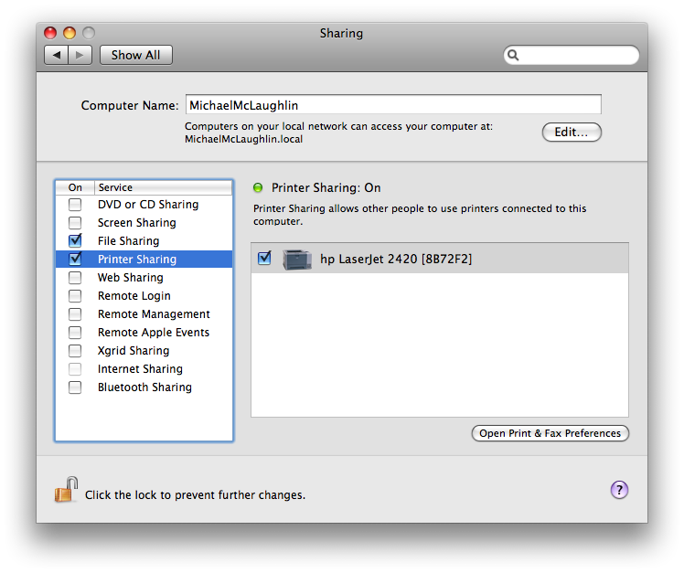
The first step requires that you share you printer setup on the Mac OS. You do that by launching System Preferences, then click on Sharing. In Sharing, you enable print sharing by chosing the network printer …
After you’ve enabled sharing on the Mac OS, you can take the following steps in Windows:
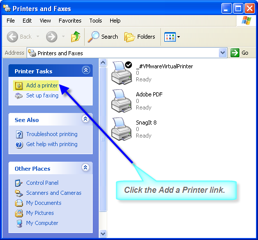
1. Click the Start button, then choose Printers and Faxes. You’ll get the following screen where you should click the link to Add a printer. It will launch the Add Print Wizard.
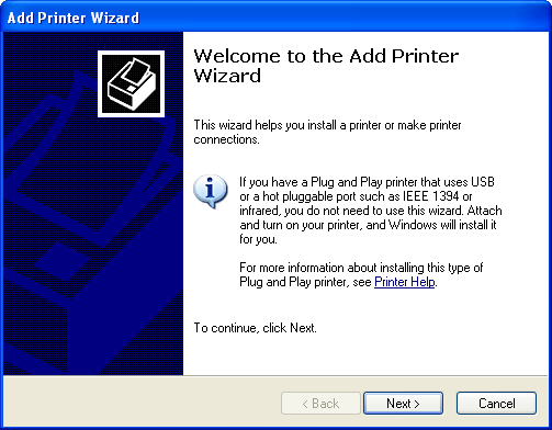
2. You should install the printer drivers if they’re not already installed before launching the Add Print Wizard. You click Next In the first screen.
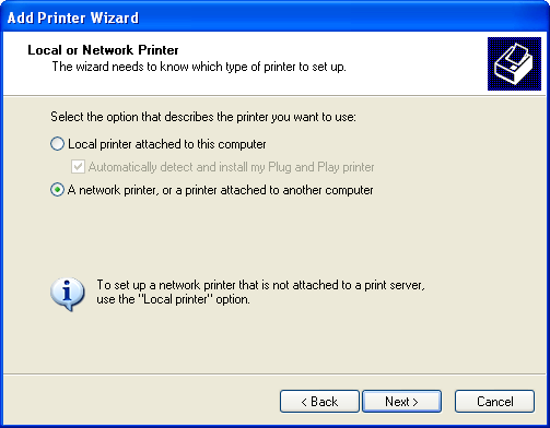
3. The default radio button is for a locally attached printer. Click the network printer radio button before clicking the Next button.
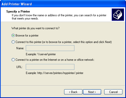
4. Click the Next button because the default browses for a network connected printer.
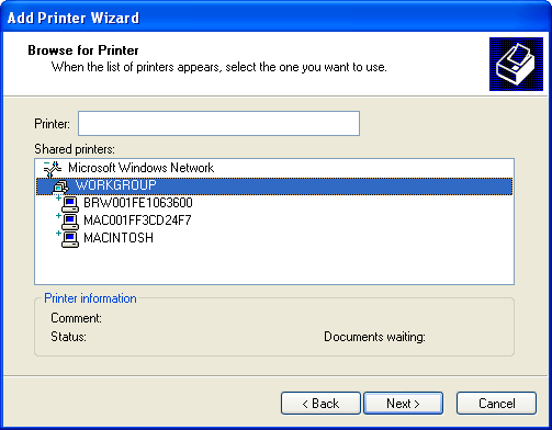
5. You shuold see the Microsoft Windows Network, and the default workgroup. Click on the Workgroup to display the possible machine names. If your machine doesn’t show in the list, it’s most likely because your printer wasn’t known in when Windows XP was released. The solution here is to insert the HP disk when you’ve connected it to the virtual machine, and then you simply follow the prompts, as shown in this newer post.
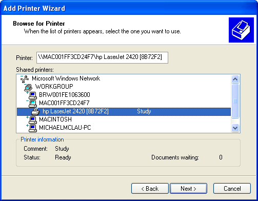
6. Click the appropriate machine that represents the hosting Mac OS (your machine that’s running VMWare). After you click it, you’ll see the target printers that are available through the external Mac OS connectivity and sharing. Click the Next button to proceed.
7. The last activity triggers a warning error. It asks you to confirm that you can trust your Mac. Click the Yes button to proceed (it’s a boring message but click on it if you want to read it).
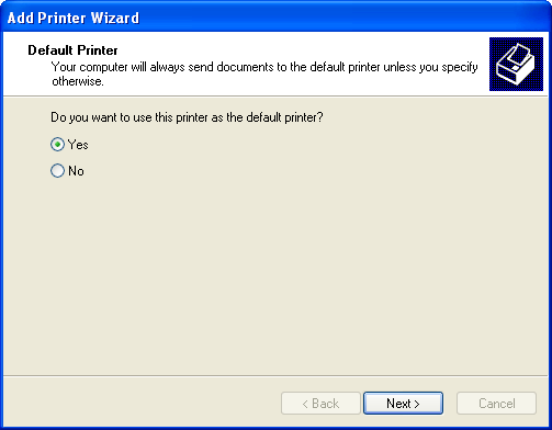
8. Choose the printer as a default printer by clicking the Yes button. You can choose the No button if you’ve got more than one network printer.
There are problems when you forget to install the hardware first, so make sure you get the hardware installed first.


