Archive for the ‘Oracle DBA’ Category
Updating Nested Tables
This two-part series covers how you update User-Defined Types (UDTs) and Attribute Data Types (ADTs). There are two varieties of UDTs. One is a column of a UDT object type and the other a UDT collection of a UDT object type.
You update nested UDT columns by leveraging the TABLE function. The TABLE function lets you create a result set, and access a UDT object or collection column. You need to combine the TABLE function and a CROSS JOIN to update elements of a UDT collection column.
ADTs are collections of a scalar data types. Oracle’s scalar data types are DATE, NUMBER, CHAR and VARCHAR2 (or, variable length strings). ADTs are unique and from some developer’s perspective difficult to work with.
The first article in this series shows you how to work with a UDT object type column and a UDT collection type. The second article will show you how to work with an ADT collection type.
PL/SQL uses ADT collections all the time. PL/SQL also uses User-Defined Types (UDTs) collections all the time. UDTs can be record or object types, or collections of records and objects. Record types are limited, and only work inside a PL/SQL scope. Object types are less limited and you can use them in a SQL or PL/SQL scope.
Object types come in two flavors. One acts as a typical record structure and has no methods and the other acts like an object type in any object-oriented programming language (OOPL). This article refers only to object types like typical record structures. That means when you read ADTs you should think of a SQL collection of a scalar data type, and when you read UDTs you should think of a SQL collection of an object type without methods.
You can create tables that hold nested tables. Nested tables can use a SQL ADT or UDT data type. Inserting data into nested tables is straightforward when you understand the syntax, but updating nested tables can be complex. The complexity exists because Oracle treats nested tables of ADTs differently than UDTs. My article series will show you how to simplify updating ADT columns.
That’s why it has two parts:
- How you insert and update rows with UDT columns and collection columns
- How you insert and update rows with ADT collection columns
If you’re asking yourself why there isn’t a section for deleting rows, that’s simple. You delete them the same way as you would any other row, using the DELETE statement.
How you insert and update rows with UDT columns and collection columns
This section shows you how to create a table with a UDT column and a UDT collection column. It also shows you how to insert and update the embedded columns.
You insert into any ordinary UDT column by prefacing the data with a constructor name. A constructor name is the same as a UDT name. The following creates an address_type UDT that you will use inside a customer table:
SQL> CREATE OR REPLACE 2 TYPE address_type IS OBJECT 3 ( street VARCHAR2(20) 4 , city VARCHAR2(30) 5 , state VARCHAR2(2) 6 , zip VARCHAR2(5)); 7 / |
You should take note that the address_type UDT doesn’t have any methods. All object types without methods have a default constructor. The default constructor follows the same rules as tables in the database.
Create the sample customer table with an address column that uses the address_type UDT as its data type; for instance:
SQL> CREATE TABLE customer 2 ( customer_id NUMBER 3 , first_name VARCHAR2(20) 4 , last_name VARCHAR2(20) 5 , address ADDRESS_TYPE 6 , CONSTRAINT pk_customer PRIMARY KEY (customer_id)); |
Line 5 defines the address column with the address_type UDT. You insert a row with an embedded address_type data record as follows:
SQL> INSERT 2 INTO customer 3 VALUES 4 ( customer_s.NEXTVAL 5 ,'Oliver' 6 ,'Queen' 7 , address_type( street => '1 Park Place' 8 , city => 'Starling City' 9 , state => 'NY' 10 , zip => '10001')); |
Lines 7 through 10 includes the constructor call to the address_type UDT. The address_type constructor uses named notation rather than positional notation. You should always try to use named notation for object type constructor calls.
Updating an element of a UDT object structure is straightforward, because you simply refer to the column and a member of the UDT object structure. The syntax for that type of UPDATE statement follows:
SQL> UPDATE customer c 2 SET c.address.state = 'NJ' 3 WHERE c.first_name = 'Oliver' 4 AND c.last_name = 'Queen'; |
The address_type UDT works for an object structure but not for a UDT collection. You need to add a column to differentiate between rows of the nested collection. You can redefine the address_type UDT as follows:
SQL> CREATE OR REPLACE 2 TYPE address_type IS OBJECT 3 ( status VARCHAR2(8) 4 , street VARCHAR2(20) 5 , city VARCHAR2(30) 6 , state VARCHAR2(2) 7 , zip VARCHAR2(5)); 8 / |
After creating the UDT object type, you need to create an address_table UDT collection of the address_type UDT object type. You use the following syntax to create the SQL collection:
SQL> CREATE OR REPLACE 2 TYPE address_table IS TABLE OF address_type; 3 / |
Having both the UDT object and collection types, you can drop and create the customer table with the following syntax:
SQL> CREATE TABLE customer 2 ( customer_id NUMBER 3 , first_name VARCHAR2(20) 4 , last_name VARCHAR2(20) 5 , address ADDRESS_TABLE 6 , CONSTRAINT pk_customer PRIMARY KEY (customer_id)) 7 NESTED TABLE address STORE AS address_tab; |
Line 5 defines the address column as a UDT collection. Line 7 instructs how to store the UDT collection as a nested table. You designate the address column as the nested table and store it as an address_tab table. You can access the nested table only through its container, which is the customer table.
You can insert rows into the customer table with the following syntax. This example stores a single row with two elements of the address_type in the nested table:
SQL> INSERT 2 INTO customer 3 VALUES 4 ( customer_s.NEXTVAL 5 ,'Oliver' 6 ,'Queen' 7 , address_table( 8 address_type( status => 'Obsolete' 9 , street => '1 Park Place' 10 , city => 'Starling City' 11 , state => 'NY' 12 , zip => '10001') 13 , address_type( status => 'Current' 14 , street => '1 Dockland Street' 15 , city => 'Starling City' 16 , state => 'NY' 17 , zip => '10001'))); |
Lines 7 through 17 have two constructor calls for the address_type UDT object type inside the address_table UDT collection. After you insert an address_table UDT collection, you can query an element by using the SQL built-in TABLE function and a CROSS JOIN. The TABLE function returns a SQL result set. The CROSS JOIN lets you create cross product that you can filter inside the WHERE clause.
A CROSS JOIN between two tables or a table and result set from a nested table matches every row in the customer table with every row in the nested table. A best practice would include a WHERE clause that filters the nested table to a single row in the result set.
The syntax for such a query is complex, and follows below:
SQL> COL first_name FORMAT A8 HEADING "First|Name" SQL> COL last_name FORMAT A8 HEADING "Last|Name" SQL> COL street FORMAT A20 HEADING "Street" SQL> COL city FORMAT A14 HEADING "City" SQL> COL state FORMAT A5 HEADING "State" SQL> SELECT c.first_name 2 , c.last_name 3 , a.street 4 , a.city 5 , a.state 6 FROM customer c CROSS JOIN TABLE(c.address) a 7 WHERE a.status = 'Current'; |
As mentioned, the TABLE function on line 6 translates the UDT collection into a SQL result set, which acts as a temporary table. The alias a becomes the name of the temporary table. Lines 3, 4, 5, and 7 all reference the temporary table.
The query should return the following for the customer and their current address value:
First Last Name Name Street City State -------- -------- -------------------- -------------- ----- Oliver Queen 1 Dockland Street Starling City NY |
Oracle thought through the fact that you should be able to update UDT collections. The same TABLE function lets you update elements in the nested table. You can update the elements in nested UDT tables provided you create a unique key, such as a natural key or primary key. Oracle’s syntax doesn’t support constraints on nested tables, which means you need to implement it by design and protect by carefully controlling inserts and updates to the nested table.
You can update the state value of the current address with the following UPDATE statement:
SQL> UPDATE TABLE(SELECT c.address 2 FROM customer c 3 WHERE c.first_name = 'Oliver' 4 AND c.last_name = 'Queen') a 5 SET a.state = 'NJ' 6 WHERE a.status = 'Current'; |
Line 5 sets the current state value in the address_table UDT nested table. Line 6 filters the nested table to the current address element. You need to ensure that any UDT object type holds a member attribute or set of member attributes that holds a unique value. That’s because you need to ensure that there’s a way to find a unique element within a UDT collection. If you require the table, you should see the change inside the nested table.
Oracle does not provide equivalent syntax for such a change in an ADT collection type. The second article in this series show you how to implement PL/SQL functions to solve that problem.
Disk Space Allocation
It’s necessary to check for adequate disk space on your Virtual Machine (VM) before installing Oracle 23c Free in a Docker container or as a podman service. Either way, it requires about 13 GB of disk space. On Ubuntu, the typical install of a VM allocates 20 GB and a 500 MB swap. You need to create a 2 GB swap when you install Ubuntu or plan to change the swap, as qualified in this excellent DigitalOcean article. Assuming you installed it with the correct swap or extended your swap area, you can confirm it with the following command:
sudo swapon --show |
It should return something like this:
NAME TYPE SIZE USED PRIO /swapfile file 2.1G 1.2G -2 |
Next, check your disk space allocation and availability with this command:
df -h |
This is what was in my instance with MySQL and PostgreSQL databases already installed and configured with sandboxed schemas:
Filesystem Size Used Avail Use% Mounted on tmpfs 388M 2.1M 386M 1% /run /dev/sda3 20G 14G 4.6G 75% / tmpfs 1.9G 28K 1.9G 1% /dev/shm tmpfs 5.0M 4.0K 5.0M 1% /run/lock /dev/sda2 512M 6.1M 506M 2% /boot/efi tmpfs 388M 108K 388M 1% /run/user/1000 |
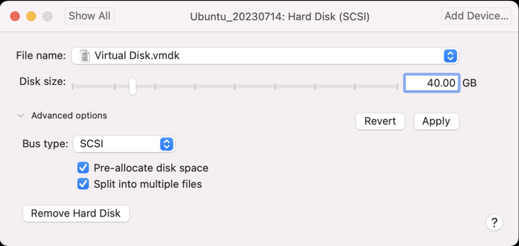
Using VMware Fusion on my Mac (Intel-based i9), I changed the allocated space from 20 GB to 40 GB by navigating to Virtual Machine, Settings…, Hard Disk. I entered 40.00 as the disk size and clicked the Pre-allocate disk space checkbox before clicking the Apply button, as shown in below. This added space is necessary because Oracle Database 23c Free as a Docker instance requires almost 10 GB of local space.
After clicking the Apply button, I checked Ubuntu with the “df -h” command and found there was no change. That’s unlike doing the same thing on AlmaLinux or a RedHat distribution, which was surprising.
The next set of steps required that I manually add the space to the Ubuntu instance:
- Start the Ubuntu VM and check the instance’s disk information with fdisk:
sudo fdisk -l
The log file for this is:
Display detailed console log →
Disk /dev/loop0: 238.77 MiB, 250372096 bytes, 489008 sectors
Units: sectors of 1 * 512 = 512 bytes
Sector size (logical/physical): 512 bytes / 512 bytes
I/O size (minimum/optimal): 512 bytes / 512 bytes


Disk /dev/loop1: 73.86 MiB, 77443072 bytes, 151256 sectors
Units: sectors of 1 * 512 = 512 bytes
Sector size (logical/physical): 512 bytes / 512 bytes
I/O size (minimum/optimal): 512 bytes / 512 bytes


Disk /dev/loop2: 349.7 MiB, 366682112 bytes, 716176 sectors
Units: sectors of 1 * 512 = 512 bytes
Sector size (logical/physical): 512 bytes / 512 bytes
I/O size (minimum/optimal): 512 bytes / 512 bytes


Disk /dev/loop3: 91.69 MiB, 96141312 bytes, 187776 sectors
Units: sectors of 1 * 512 = 512 bytes
Sector size (logical/physical): 512 bytes / 512 bytes
I/O size (minimum/optimal): 512 bytes / 512 bytes


Disk /dev/loop4: 496.98 MiB, 521121792 bytes, 1017816 sectors
Units: sectors of 1 * 512 = 512 bytes
Sector size (logical/physical): 512 bytes / 512 bytes
I/O size (minimum/optimal): 512 bytes / 512 bytes


Disk /dev/loop5: 45.93 MiB, 48160768 bytes, 94064 sectors
Units: sectors of 1 * 512 = 512 bytes
Sector size (logical/physical): 512 bytes / 512 bytes
I/O size (minimum/optimal): 512 bytes / 512 bytes


Disk /dev/loop6: 128.92 MiB, 135184384 bytes, 264032 sectors
Units: sectors of 1 * 512 = 512 bytes
Sector size (logical/physical): 512 bytes / 512 bytes
I/O size (minimum/optimal): 512 bytes / 512 bytes


Disk /dev/loop7: 63.45 MiB, 66531328 bytes, 129944 sectors
Units: sectors of 1 * 512 = 512 bytes
Sector size (logical/physical): 512 bytes / 512 bytes
I/O size (minimum/optimal): 512 bytes / 512 bytes


Disk /dev/fd0: 1.41 MiB, 1474560 bytes, 2880 sectors
Units: sectors of 1 * 512 = 512 bytes
Sector size (logical/physical): 512 bytes / 512 bytes
I/O size (minimum/optimal): 512 bytes / 512 bytes
Disklabel type: dos
Disk identifier: 0x90909090

Device     Boot      Start        End    Sectors  Size Id Type
/dev/fd0p1      2425393296 4850786591 2425393296  1.1T 90 unknown
/dev/fd0p2      2425393296 4850786591 2425393296  1.1T 90 unknown
/dev/fd0p3      2425393296 4850786591 2425393296  1.1T 90 unknown
/dev/fd0p4      2425393296 4850786591 2425393296  1.1T 90 unknown
GPT PMBR size mismatch (41943039 != 83886079) will be corrected by write.


Disk /dev/sda: 40 GiB, 42949672960 bytes, 83886080 sectors
Disk model: VMware Virtual S
Units: sectors of 1 * 512 = 512 bytes
Sector size (logical/physical): 512 bytes / 512 bytes
I/O size (minimum/optimal): 512 bytes / 512 bytes
Disklabel type: gpt
Disk identifier: 7906AE0B-498C-4FE4-8B45-9CD1B2265197

Device       Start      End  Sectors  Size Type
/dev/sda1     2048     4095     2048    1M BIOS boot
/dev/sda2     4096  1054719  1050624  513M EFI System
/dev/sda3  1054720 41940991 40886272 19.5G Linux filesystem


Disk /dev/loop8: 40.84 MiB, 42827776 bytes, 83648 sectors
Units: sectors of 1 * 512 = 512 bytes
Sector size (logical/physical): 512 bytes / 512 bytes
I/O size (minimum/optimal): 512 bytes / 512 bytes


Disk /dev/loop9: 304 KiB, 311296 bytes, 608 sectors
Units: sectors of 1 * 512 = 512 bytes
Sector size (logical/physical): 512 bytes / 512 bytes
I/O size (minimum/optimal): 512 bytes / 512 bytes


Disk /dev/loop10: 452 KiB, 462848 bytes, 904 sectors
Units: sectors of 1 * 512 = 512 bytes
Sector size (logical/physical): 512 bytes / 512 bytes
I/O size (minimum/optimal): 512 bytes / 512 bytes


Disk /dev/loop13: 496.88 MiB, 521015296 bytes, 1017608 sectors
Units: sectors of 1 * 512 = 512 bytes
Sector size (logical/physical): 512 bytes / 512 bytes
I/O size (minimum/optimal): 512 bytes / 512 bytes


Disk /dev/loop12: 240.05 MiB, 251707392 bytes, 491616 sectors
Units: sectors of 1 * 512 = 512 bytes
Sector size (logical/physical): 512 bytes / 512 bytes
I/O size (minimum/optimal): 512 bytes / 512 bytes


Disk /dev/loop11: 4 KiB, 4096 bytes, 8 sectors
Units: sectors of 1 * 512 = 512 bytes
Sector size (logical/physical): 512 bytes / 512 bytes
I/O size (minimum/optimal): 512 bytes / 512 bytes


Disk /dev/loop14: 346.33 MiB, 363151360 bytes, 709280 sectors
Units: sectors of 1 * 512 = 512 bytes
Sector size (logical/physical): 512 bytes / 512 bytes
I/O size (minimum/optimal): 512 bytes / 512 bytes


Disk /dev/loop16: 12.32 MiB, 12922880 bytes, 25240 sectors
Units: sectors of 1 * 512 = 512 bytes
Sector size (logical/physical): 512 bytes / 512 bytes
I/O size (minimum/optimal): 512 bytes / 512 bytes


Disk /dev/loop17: 73.9 MiB, 77492224 bytes, 151352 sectors
Units: sectors of 1 * 512 = 512 bytes
Sector size (logical/physical): 512 bytes / 512 bytes
I/O size (minimum/optimal): 512 bytes / 512 bytes


Disk /dev/loop15: 175.83 MiB, 184373248 bytes, 360104 sectors
Units: sectors of 1 * 512 = 512 bytes
Sector size (logical/physical): 512 bytes / 512 bytes
I/O size (minimum/optimal): 512 bytes / 512 bytes


Disk /dev/loop18: 63.46 MiB, 66547712 bytes, 129976 sectors
Units: sectors of 1 * 512 = 512 bytes
Sector size (logical/physical): 512 bytes / 512 bytes
I/O size (minimum/optimal): 512 bytes / 512 bytes


Disk /dev/loop19: 40.86 MiB, 42840064 bytes, 83672 sectors
Units: sectors of 1 * 512 = 512 bytes
Sector size (logical/physical): 512 bytes / 512 bytes
I/O size (minimum/optimal): 512 bytes / 512 bytes
After running fdisk, I rechecked disk allocation with df -h and saw no change:
Filesystem      Size  Used Avail Use% Mounted on
tmpfs           388M  2.1M  386M   1% /run
/dev/sda3        20G   14G  4.6G  75% /
tmpfs           1.9G   28K  1.9G   1% /dev/shm
tmpfs           5.0M  4.0K  5.0M   1% /run/lock
/dev/sda2       512M  6.1M  506M   2% /boot/efi
tmpfs           388M  108K  388M   1% /run/user/1000
- So, I installed Ubuntu’s user space utility gparted:
sudo apt install gparted
The log file for this is:
Display detailed console log →
Reading package lists... Done
Building dependency tree... Done
Reading state information... Done
The following additional packages will be installed:
  gparted-common
Suggested packages:
  dmraid gpart jfsutils kpartx mtools reiser4progs reiserfsprogs udftools
  xfsprogs exfatprogs
The following NEW packages will be installed:
  gparted gparted-common
0 upgraded, 2 newly installed, 0 to remove and 4 not upgraded.
Need to get 490 kB of archives.
After this operation, 2,128 kB of additional disk space will be used.
Do you want to continue? [Y/n] Y
Get:1 http://us.archive.ubuntu.com/ubuntu jammy/main amd64 gparted-common all 1.3.1-1ubuntu1 [71.9 kB]
Get:2 http://us.archive.ubuntu.com/ubuntu jammy/main amd64 gparted amd64 1.3.1-1ubuntu1 [418 kB]
Fetched 490 kB in 2s (211 kB/s)
Selecting previously unselected package gparted-common.
(Reading database ... 203026 files and directories currently installed.)
Preparing to unpack .../gparted-common_1.3.1-1ubuntu1_all.deb ...
Unpacking gparted-common (1.3.1-1ubuntu1) ...
Selecting previously unselected package gparted.
Preparing to unpack .../gparted_1.3.1-1ubuntu1_amd64.deb ...
Unpacking gparted (1.3.1-1ubuntu1) ...
Setting up gparted-common (1.3.1-1ubuntu1) ...
Setting up gparted (1.3.1-1ubuntu1) ...
Processing triggers for mailcap (3.70+nmu1ubuntu1) ...
Processing triggers for desktop-file-utils (0.26-1ubuntu3) ...
Processing triggers for hicolor-icon-theme (0.17-2) ...
Processing triggers for gnome-menus (3.36.0-1ubuntu3) ...
Processing triggers for man-db (2.10.2-1) ...
- After installing the gparted utility (manual can be found here), you can launch it with the following syntax:
sudo gpartedYou’ll see the following in the console, which you can ignore.
GParted 1.3.1
configuration --enable-libparted-dmraid --enable-online-resize
libparted 3.4
It launches a GUI interface that should look something like the following:
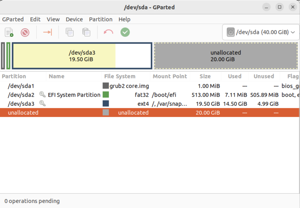
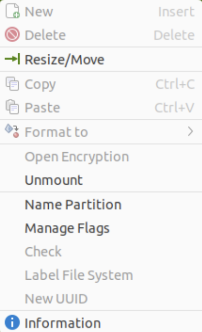
Right-click on the /dev/sda3 Partition and the GParted application will present the following context popup menu. Click the Resize/Move menu option.
The attempt to resize the disk at this point GParted will raise a read-only exception like the following:
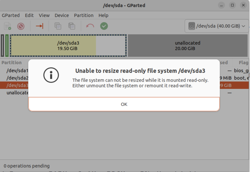
You might open a new shell and fix the disk at the command-line but you’ll need to relaunch gparted regardless. So, you should close gparted and run the following commands:
sudo mount -o remount -rw /
sudo mount -o remount -rw /var/snap/firefox/common/host-hunspell
When you relaunch GParted, you see that the graphic depiction has changed when you right-click on the /dev/sda3 Partition as follows:
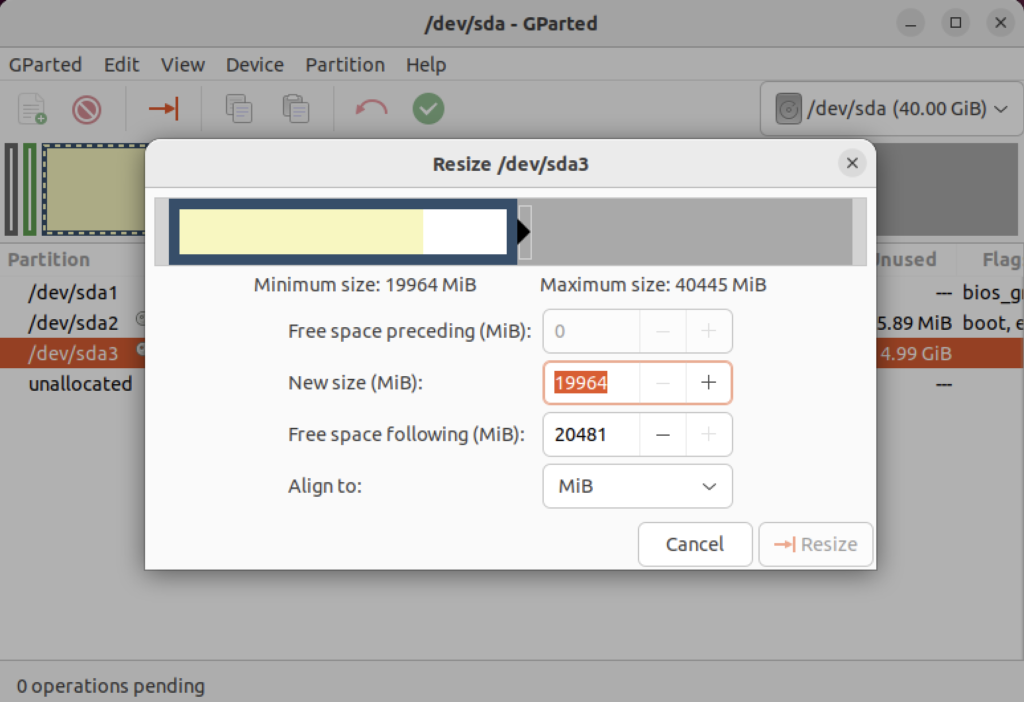
Click on the highlighted box with the arrow and drag it all the way to the right. It will then show you something like the following.
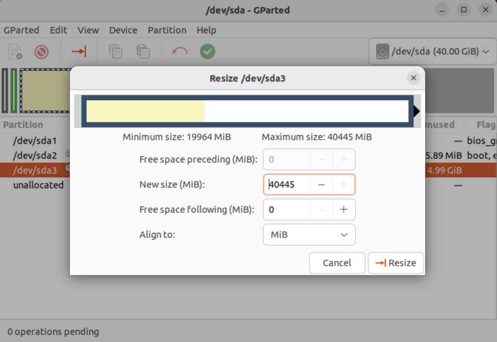
Click the Resize button to make the change and add the space to the Ubuntu file system and see something like the following in Gparted:
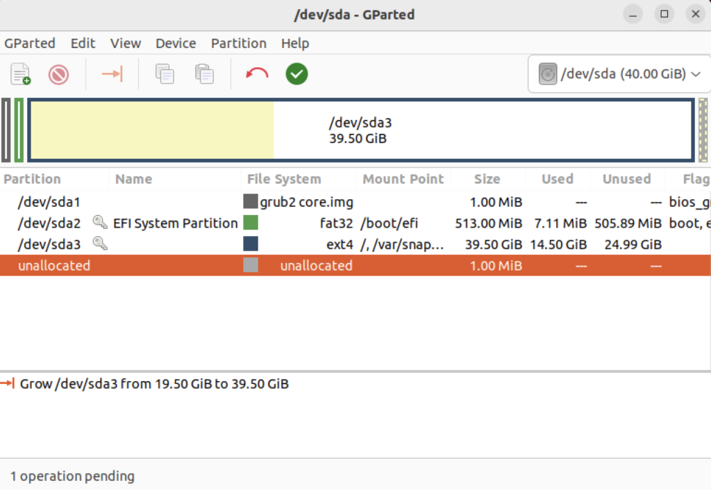
Choose Edit in the menu bar and then Apply All Operations to effect the change in the disk allocation. The last dialog will require you to verify you want to make the changes. Click the Apply button to make the changes.
Click the close for the GParted application and then you can rerun the following command:
df -h
You will see that you now have 19.5 GB of additional space:
Filesystem      Size  Used Avail Use% Mounted on
tmpfs           388M  2.2M  386M   1% /run
/dev/sda3        39G 19.5G   23G  39% /
tmpfs           1.9G   28K  1.9G   1% /dev/shm
tmpfs           5.0M  4.0K  5.0M   1% /run/lock
/dev/sda2       512M  6.1M  506M   2% /boot/efi
tmpfs           388M  116K  388M   1% /run/user/1000
- Finally, you can now successfully download the latest Docker version of Oracle Database 23c Free with the following command:
docker run --name oracle23c -p 1521:1521 -p 5500:5500 -e ORACLE_PWD=cangetin container-registry.oracle.com/database/free:latest
Since you haven’t downloaded the container, you’ll get a warning that it is unable to find the image before it discovers it and downloads it. This will take several minutes. At the conclusion, it will start the Oracle Database Net Listener and begin updating files. the updates may take quite a while to complete.
The basic download console output looks like the following and if you check your disk space you’ve downloaded about 14 GB in the completed container.
Unable to find image 'container-registry.oracle.com/database/free:latest' locally
latest: Pulling from database/free
089fdfcd47b7: Pull complete
43c899d88edc: Pull complete
47aa6f1886a1: Pull complete
f8d07bb55995: Pull complete
c31c8c658c1e: Pull complete
b7d28faa08b4: Pull complete
1d0d5c628f6f: Pull complete
db82a695dad3: Pull complete
25a185515793: Pull complete
Digest: sha256:5ac0efa9896962f6e0e91c54e23c03ae8f140cf6ed43ca09ef4354268a942882
Status: Downloaded newer image for container-registry.oracle.com/database/free:latest
My detailed log file for the complete recovery operation is:
Display detailed console log →
Starting Oracle Net Listener.
Oracle Net Listener started.
Starting Oracle Database instance FREE.
Oracle Database instance FREE started.

The Oracle base remains unchanged with value /opt/oracle

SQL*Plus: Release 23.0.0.0.0 - Production on Thu Nov 30 22:40:55 2023
Version 23.3.0.23.09

Copyright (c) 1982, 2023, Oracle.  All rights reserved.


Connected to:
Oracle Database 23c Free Release 23.0.0.0.0 - Develop, Learn, and Run for Free
Version 23.3.0.23.09

SQL>
User altered.

SQL>
User altered.

SQL>
Session altered.

SQL>
User altered.

SQL> Disconnected from Oracle Database 23c Free Release 23.0.0.0.0 - Develop, Learn, and Run for Free
Version 23.3.0.23.09
The Oracle base remains unchanged with value /opt/oracle
#########################
DATABASE IS READY TO USE!
#########################
The following output is now a tail of the alert.log:
Completed: Pluggable database FREEPDB1 opened read write
Completed: ALTER DATABASE OPEN
2023-11-30T22:40:55.538359+00:00
===========================================================
Dumping current patch information
===========================================================
No patches have been applied
===========================================================
2023-11-30T22:40:57.521629+00:00
FREEPDB1(3):TABLE AUDSYS.AUD$UNIFIED: ADDED INTERVAL PARTITION SYS_P342 (3440) VALUES LESS THAN (TIMESTAMP' 2023-12-01 00:00:00')
2023-11-30T22:41:00.565540+00:00
TABLE SYS.WRP$_REPORTS: ADDED AUTOLIST FRAGMENT SYS_P413 (3) VALUES (( 1418518649, TO_DATE(' 2023-11-27 00:00:00', 'syyyy-mm-dd hh24:mi:ss', 'nls_calendar=gregorian') ))
TABLE SYS.WRP$_REPORTS_DETAILS: ADDED AUTOLIST FRAGMENT SYS_P414 (3) VALUES (( 1418518649, TO_DATE(' 2023-11-27 00:00:00', 'syyyy-mm-dd hh24:mi:ss', 'nls_calendar=gregorian') ))
TABLE SYS.WRP$_REPORTS_TIME_BANDS: ADDED AUTOLIST FRAGMENT SYS_P417 (3) VALUES (( 1418518649, TO_DATE(' 2023-11-27 00:00:00', 'syyyy-mm-dd hh24:mi:ss', 'nls_calendar=gregorian') ))
2023-11-30T22:41:45.639208+00:00
FREEPDB1(3):Resize operation completed for file# 13, fname /opt/oracle/oradata/FREE/FREEPDB1/sysaux01.dbf, old size 317440K, new size 327680K
2023-11-30T22:41:45.663044+00:00
FREEPDB1(3):Resize operation completed for file# 13, fname /opt/oracle/oradata/FREE/FREEPDB1/sysaux01.dbf, old size 327680K, new size 337920K
2023-11-30T22:46:51.616417+00:00
Resize operation completed for file# 201, fname /opt/oracle/oradata/FREE/temp01.dbf, old size 20480K, new size 86016K
Resize operation completed for file# 201, fname /opt/oracle/oradata/FREE/temp01.dbf, old size 86016K, new size 151552K
Resize operation completed for file# 201, fname /opt/oracle/oradata/FREE/temp01.dbf, old size 151552K, new size 217088K
2023-11-30T22:46:53.024736+00:00
Resize operation completed for file# 201, fname /opt/oracle/oradata/FREE/temp01.dbf, old size 217088K, new size 282624K
Resize operation completed for file# 201, fname /opt/oracle/oradata/FREE/temp01.dbf, old size 282624K, new size 348160K
2023-11-30T22:50:45.816010+00:00
Resize operation completed for file# 3, fname /opt/oracle/oradata/FREE/sysaux01.dbf, old size 573440K, new size 593920K
2023-11-30T23:00:46.159283+00:00
Resize operation completed for file# 3, fname /opt/oracle/oradata/FREE/sysaux01.dbf, old size 593920K, new size 604160K
2023-11-30T23:00:46.228087+00:00
FREEPDB1(3):Resize operation completed for file# 13, fname /opt/oracle/oradata/FREE/FREEPDB1/sysaux01.dbf, old size 337920K, new size 358400K
2023-12-01T00:30:43.494249+00:00
--ATTENTION--
Heavy swapping observed on system
WARNING: Heavy swapping observed on system in last 5 mins.
Heavy swapping can lead to timeouts, poor performance, and instance eviction.
2023-12-01T12:40:07.820678+00:00
Warning: VKTM detected a forward time drift.
Please see the VKTM trace file for more details:
/opt/oracle/diag/rdbms/free/FREE/trace/FREE_vktm_46.trc
2023-12-01T16:09:32.702179+00:00
Warning: VKTM detected a forward time drift.
Time drifts can result in unexpected behavior such as time-outs.
Please see the VKTM trace file for more details:
/opt/oracle/diag/rdbms/free/FREE/trace/FREE_vktm_46.trc
2023-12-01T18:02:02.658867+00:00
FREEPDB1(3):Resize operation completed for file# 13, fname /opt/oracle/oradata/FREE/FREEPDB1/sysaux01.dbf, old size 358400K, new size 368640K
2023-12-01T18:22:03.858970+00:00
Resize operation completed for file# 3, fname /opt/oracle/oradata/FREE/sysaux01.dbf, old size 604160K, new size 624640K
2023-12-01T20:31:39.671144+00:00
Warning: VKTM detected a forward time drift.
Time drifts can result in unexpected behavior such as time-outs.
Please see the VKTM trace file for more details:
/opt/oracle/diag/rdbms/free/FREE/trace/FREE_vktm_46.trc
2023-12-01T22:16:50.007797+00:00
Warning: VKTM detected a forward time drift.
Time drifts can result in unexpected behavior such as time-outs.
Please see the VKTM trace file for more details:
/opt/oracle/diag/rdbms/free/FREE/trace/FREE_vktm_46.trc
2023-12-01T23:11:39.776733+00:00
Resize operation completed for file# 3, fname /opt/oracle/oradata/FREE/sysaux01.dbf, old size 624640K, new size 634880K
2023-12-01T23:11:39.920882+00:00
FREEPDB1(3):Resize operation completed for file# 13, fname /opt/oracle/oradata/FREE/FREEPDB1/sysaux01.dbf, old size 368640K, new size 378880K
2023-12-01T23:11:45.530407+00:00
Begin automatic SQL Tuning Advisor run for special tuning task "SYS_AUTO_SQL_TUNING_TASK".
2023-12-01T23:11:46.626668+00:00
End automatic SQL Tuning Advisor run for special tuning task "SYS_AUTO_SQL_TUNING_TASK".
2023-12-01T23:11:56.518724+00:00
TABLE SYS.WRI$_OPTSTAT_HISTHEAD_HISTORY: ADDED INTERVAL PARTITION SYS_P473 (45260) VALUES LESS THAN (TO_DATE(' 2023-12-02 00:00:00', 'SYYYY-MM-DD HH24:MI:SS', 'NLS_CALENDAR=GREGORIAN'))
TABLE SYS.WRI$_OPTSTAT_HISTGRM_HISTORY: ADDED INTERVAL PARTITION SYS_P476 (45260) VALUES LESS THAN (TO_DATE(' 2023-12-02 00:00:00', 'SYYYY-MM-DD HH24:MI:SS', 'NLS_CALENDAR=GREGORIAN'))
2023-12-01T23:13:58.659641+00:00
Resize operation completed for file# 1, fname /opt/oracle/oradata/FREE/system01.dbf, old size 1085440K, new size 1095680K
2023-12-01T23:14:27.016016+00:00
Thread 1 advanced to log sequence 3 (LGWR switch),  current SCN: 3248652
  Current log# 3 seq# 3 mem# 0: /opt/oracle/oradata/FREE/redo03.log
2023-12-01T23:14:47.256059+00:00
cellip.ora not found.
2023-12-01T23:14:54.365395+00:00
Resize operation completed for file# 11, fname /opt/oracle/oradata/FREE/undotbs01.dbf, old size 40960K, new size 46080K
Resize operation completed for file# 11, fname /opt/oracle/oradata/FREE/undotbs01.dbf, old size 46080K, new size 51200K
2023-12-01T23:16:40.460917+00:00
--ATTENTION--
Heavy swapping observed on system
WARNING: Heavy swapping observed on system in last 5 mins.
Heavy swapping can lead to timeouts, poor performance, and instance eviction.
2023-12-02T11:40:23.802013+00:00
Warning: VKTM detected a forward time drift.
Please see the VKTM trace file for more details:
/opt/oracle/diag/rdbms/free/FREE/trace/FREE_vktm_46.trc
2023-12-02T11:40:24.917287+00:00
Warning: VKTM detected a forward time drift.
Time drifts can result in unexpected behavior such as time-outs.
Please see the VKTM trace file for more details:
/opt/oracle/diag/rdbms/free/FREE/trace/FREE_vktm_46.trc
2023-12-02T11:40:34.601396+00:00
TABLE SYS.ACTIVITY_TABLE$: ADDED INTERVAL PARTITION SYS_P493 (2) VALUES LESS THAN (202)
2023-12-02T19:35:06.380899+00:00
Warning: VKTM detected a forward time drift.
Time drifts can result in unexpected behavior such as time-outs.
Please see the VKTM trace file for more details:
/opt/oracle/diag/rdbms/free/FREE/trace/FREE_vktm_46.trc
2023-12-02T19:35:11.094760+00:00
Begin automatic SQL Tuning Advisor run for special tuning task "SYS_AUTO_SQL_TUNING_TASK".
2023-12-02T19:35:11.913190+00:00
FREEPDB1(3):TABLE SYS.WRI$_OPTSTAT_HISTHEAD_HISTORY: ADDED INTERVAL PARTITION SYS_P442 (45261) VALUES LESS THAN (TO_DATE(' 2023-12-03 00:00:00', 'SYYYY-MM-DD HH24:MI:SS', 'NLS_CALENDAR=GREGORIAN'))
FREEPDB1(3):TABLE SYS.WRI$_OPTSTAT_HISTGRM_HISTORY: ADDED INTERVAL PARTITION SYS_P445 (45261) VALUES LESS THAN (TO_DATE(' 2023-12-03 00:00:00', 'SYYYY-MM-DD HH24:MI:SS', 'NLS_CALENDAR=GREGORIAN'))
2023-12-02T19:35:12.623823+00:00
FREEPDB1(3):TABLE SYS.ACTIVITY_TABLE$: ADDED INTERVAL PARTITION SYS_P446 (2) VALUES LESS THAN (202)
2023-12-02T19:35:15.630900+00:00
End automatic SQL Tuning Advisor run for special tuning task "SYS_AUTO_SQL_TUNING_TASK".
2023-12-02T19:35:26.656198+00:00
TABLE SYS.WRI$_OPTSTAT_HISTHEAD_HISTORY: ADDED INTERVAL PARTITION SYS_P513 (45261) VALUES LESS THAN (TO_DATE(' 2023-12-03 00:00:00', 'SYYYY-MM-DD HH24:MI:SS', 'NLS_CALENDAR=GREGORIAN'))
TABLE SYS.WRI$_OPTSTAT_HISTGRM_HISTORY: ADDED INTERVAL PARTITION SYS_P516 (45261) VALUES LESS THAN (TO_DATE(' 2023-12-03 00:00:00', 'SYYYY-MM-DD HH24:MI:SS', 'NLS_CALENDAR=GREGORIAN'))
2023-12-02T19:36:00.842540+00:00
FREEPDB1(3):TABLE SYS.WRP$_REPORTS: ADDED AUTOLIST FRAGMENT SYS_P482 (2) VALUES (( 2054829351, TO_DATE(' 2023-11-27 00:00:00', 'syyyy-mm-dd hh24:mi:ss', 'nls_calendar=gregorian') ))
FREEPDB1(3):TABLE SYS.WRP$_REPORTS_DETAILS: ADDED AUTOLIST FRAGMENT SYS_P483 (2) VALUES (( 2054829351, TO_DATE(' 2023-11-27 00:00:00', 'syyyy-mm-dd hh24:mi:ss', 'nls_calendar=gregorian') ))
FREEPDB1(3):TABLE SYS.WRP$_REPORTS_TIME_BANDS: ADDED AUTOLIST FRAGMENT SYS_P486 (2) VALUES (( 2054829351, TO_DATE(' 2023-11-27 00:00:00', 'syyyy-mm-dd hh24:mi:ss', 'nls_calendar=gregorian') ))
2023-12-02T19:36:49.488283+00:00
cellip.ora not found.
2023-12-02T19:36:59.941785+00:00
FREEPDB1(3):Resize operation completed for file# 12, fname /opt/oracle/oradata/FREE/FREEPDB1/system01.dbf, old size 286720K, new size 296960K
2023-12-02T19:38:11.214065+00:00
FREEPDB1(3):cellip.ora not found.
2023-12-02T19:39:38.144241+00:00
Resize operation completed for file# 3, fname /opt/oracle/oradata/FREE/sysaux01.dbf, old size 634880K, new size 645120K
2023-12-02T19:39:38.254317+00:00
FREEPDB1(3):Resize operation completed for file# 13, fname /opt/oracle/oradata/FREE/FREEPDB1/sysaux01.dbf, old size 378880K, new size 389120K
2023-12-02T19:39:45.971914+00:00
--ATTENTION--
Heavy swapping observed on system
WARNING: Heavy swapping observed on system in last 5 mins.
Heavy swapping can lead to timeouts, poor performance, and instance eviction.
2023-12-02T19:49:39.226372+00:00
Resize operation completed for file# 3, fname /opt/oracle/oradata/FREE/sysaux01.dbf, old size 645120K, new size 655360K
2023-12-02T19:49:55.006771+00:00
Thread 1 cannot allocate new log, sequence 4
Private strand flush not complete
  Current log# 3 seq# 3 mem# 0: /opt/oracle/oradata/FREE/redo03.log
2023-12-02T19:49:58.006305+00:00
Thread 1 advanced to log sequence 4 (LGWR switch),  current SCN: 3327607
  Current log# 1 seq# 4 mem# 0: /opt/oracle/oradata/FREE/redo01.log
2023-12-02T19:51:10.096706+00:00
cellip.ora not found.
2023-12-02T19:59:39.923548+00:00
Resize operation completed for file# 3, fname /opt/oracle/oradata/FREE/sysaux01.dbf, old size 655360K, new size 665600K
2023-12-02T23:44:23.322751+00:00
Warning: VKTM detected a forward time drift.
Time drifts can result in unexpected behavior such as time-outs.
Please see the VKTM trace file for more details:
/opt/oracle/diag/rdbms/free/FREE/trace/FREE_vktm_46.trc
2023-12-03T01:20:19.592589+00:00
Warning: VKTM detected a forward time drift.
Time drifts can result in unexpected behavior such as time-outs.
Please see the VKTM trace file for more details:
/opt/oracle/diag/rdbms/free/FREE/trace/FREE_vktm_46.trc
2023-12-03T01:25:01.817094+00:00
FREEPDB1(3):Resize operation completed for file# 13, fname /opt/oracle/oradata/FREE/FREEPDB1/sysaux01.dbf, old size 389120K, new size 399360K
2023-12-03T01:25:11.199280+00:00
TABLE SYS.WRI$_OPTSTAT_HISTHEAD_HISTORY: ADDED INTERVAL PARTITION SYS_P553 (45262) VALUES LESS THAN (TO_DATE(' 2023-12-04 00:00:00', 'SYYYY-MM-DD HH24:MI:SS', 'NLS_CALENDAR=GREGORIAN'))
TABLE SYS.WRI$_OPTSTAT_HISTGRM_HISTORY: ADDED INTERVAL PARTITION SYS_P556 (45262) VALUES LESS THAN (TO_DATE(' 2023-12-04 00:00:00', 'SYYYY-MM-DD HH24:MI:SS', 'NLS_CALENDAR=GREGORIAN'))
2023-12-03T01:25:13.434023+00:00
FREEPDB1(3):TABLE SYS.WRI$_OPTSTAT_HISTHEAD_HISTORY: ADDED INTERVAL PARTITION SYS_P502 (45262) VALUES LESS THAN (TO_DATE(' 2023-12-04 00:00:00', 'SYYYY-MM-DD HH24:MI:SS', 'NLS_CALENDAR=GREGORIAN'))
FREEPDB1(3):TABLE SYS.WRI$_OPTSTAT_HISTGRM_HISTORY: ADDED INTERVAL PARTITION SYS_P505 (45262) VALUES LESS THAN (TO_DATE(' 2023-12-04 00:00:00', 'SYYYY-MM-DD HH24:MI:SS', 'NLS_CALENDAR=GREGORIAN'))
2023-12-03T01:26:29.620704+00:00
FREEPDB1(3):cellip.ora not found.
2023-12-03T01:26:36.758289+00:00
cellip.ora not found.
2023-12-03T02:25:52.946809+00:00
Warning: VKTM detected a forward time drift.
Time drifts can result in unexpected behavior such as time-outs.
Please see the VKTM trace file for more details:
/opt/oracle/diag/rdbms/free/FREE/trace/FREE_vktm_46.trc
2023-12-03T02:27:56.055089+00:00
--ATTENTION--
Heavy swapping observed on system
WARNING: Heavy swapping observed on system in last 5 mins.
Heavy swapping can lead to timeouts, poor performance, and instance eviction.
2023-12-03T02:32:47.996105+00:00
Resize operation completed for file# 3, fname /opt/oracle/oradata/FREE/sysaux01.dbf, old size 665600K, new size 675840K
You can connect to the Oracle Database 23c Free container with the following syntax:
docker exec -it -u root oracle23c bash |
At the command-line, you connect to the Oracle Database 23c Free container with the following syntax:
sqlplus system/cangetin@free |
You have arrived at the Oracle SQL prompt:
SQL*Plus: Release 23.0.0.0.0 - Production on Fri Dec 1 00:13:55 2023 Version 23.3.0.23.09 Copyright (c) 1982, 2023, Oracle. All rights reserved. Last Successful login time: Thu Nov 30 2023 23:27:54 +00:00 Connected to: Oracle Database 23c Free Release 23.0.0.0.0 - Develop, Learn, and Run for Free Version 23.3.0.23.09 SQL> |
As always, I hope this helps those trying to work with the newest Oracle stack.
AWS EC2 TNS Listener
Having configured an AlmaLinux 8.6 with Oracle Database 11g XE, MySQL 8.0.30, and PostgreSQL 15, we migrated it to AWS EC2 and provisioned it. We used the older and de-supported Oracle Database 11g XE because it didn’t require any kernel modifications and had a much smaller footprint.
I had to address why attempting to connect with the sqlplus utility raised the following error after provisioning a copy with a new static IP address:
ERROR: ORA-12514: TNS:listener does NOT currently know OF service requested IN CONNECT descriptor |
A connection from SQL Developer raises a more addressable error, like:
ORA-17069 |
I immediately tried to check the connection with the tnsping utility and found that tnsping worked fine. However, when I tried to connect with the sqlplus utility it raised an ORA-12514 connection error.
There were no diagnostic steps beyond checking the tnsping utility. So, I had to experiment with what might block communication.
I changed the host name from ip-172-58-65-82.us-west-2.compute.internal to a localhost string in both the listener.ora and tnsnames.ora. The listener.ora file:
# listener.ora Network Configuration FILE: SID_LIST_LISTENER = (SID_LIST = (SID_DESC = (SID_NAME = PLSExtProc) (ORACLE_HOME = /u01/app/oracle/product/11.2.0/xe) (PROGRAM = extproc) ) ) LISTENER = (DESCRIPTION_LIST = (DESCRIPTION = (ADDRESS = (PROTOCOL = IPC)(KEY = EXTPROC_FOR_XE)) (ADDRESS = (PROTOCOL = TCP)(HOST = localhost)(PORT = 1521)) ) ) DEFAULT_SERVICE_LISTENER = (XE) |
The tnsnames.ora file:
# tnsnames.ora Network Configuration FILE: XE = (DESCRIPTION = (ADDRESS = (PROTOCOL = TCP)(HOST = localhost)(PORT = 1521)) (CONNECT_DATA = (SERVER = DEDICATED) (SERVICE_NAME = XE) ) ) EXTPROC_CONNECTION_DATA = (DESCRIPTION = (ADDRESS_LIST = (ADDRESS = (PROTOCOL = IPC)(KEY = EXTPROC_FOR_XE)) ) (CONNECT_DATA = (SID = PLSExtProc) (PRESENTATION = RO) ) ) |
I suspected that it might be related to the localhost value. So, I checked the /etc/hostname and /etc/hosts files.
Then, I modified /etc/hostname file by removing the AWS EC2 damain address. I did it on a memory that Oracle’s TNS raises errors for dots or periods in some addresses.
The /etc/hostname file:
ip-172-58-65-82 |
The /etc/hosts file:
127.0.0.1 localhost localhost.localdomain localhost4 localhost4.localdomain4 ip-172-58-65-82 ::1 localhost localhost.localdomain localhost6 localhost6.localdomain6 ip-172-58-65-82 |
Now, we can connect to the Oracle Database 11g XE instance with the sqlplus utility. I believe this type of solution will work for other AWS EC2 provisioned Oracle databases.
AlmaLinux Install & Configuration

This is a collection of blog posts for installing and configuring AlmaLinux with the Oracle, PostgreSQL, MySQL databases and several programming languages. Sample programs show how to connect PHP and Python to the MySQL database.
- Installing AlmaLinux operating system
- Installing and configuring MySQL
- Installing Python-MySQL connector and provide sample programs
- Configuring Flask for Python on AlmaLinux with a complete software router instruction set.
- Installing Rust programming language and writing a sample program
- Installing and configuring LAMP stack with PHP and MySQL and a self-signed security key
- MySQL PNG Images in LAMP with PHP Programming
- Demonstration of how to write Perl that connects to MySQL
- Installing and configuring MySQL Workbench
- Installing and configuring PostgreSQL and pgAdmin4
- Identifying the required libnsl2-devel packages for SQL*Plus
- Writing and deploying a sqlplus function to use a read line wrapper
- Installing and configuring Visual Studio Code Editor
- Installing and configuring Java with connectivity to MySQL
- Installing and configuring Oracle SQL Developer
I used Oracle Database 11g XE in this instance to keep the footprint as small as possible. It required a few tricks and discovering the missing library that caused folks grief eleven years ago. I build another with a current Oracle Database XE after the new year.
If you see something that I missed or you’d like me to add, let me know. As time allows, I’ll try to do that. Naturally, the post will get updates as things are added later.
PL/SQL List to Struct
Every now and then, I get questions from folks about how to tune in-memory elements of their PL/SQL programs. This blog post address one of those core issues that some PL/SQL programmers avoid.
Specifically, it addresses how to convert a list of values into a structure (in C/C++ its a struct, in Java its an ArrayList, and PL/SQL it’s a table of scalar or object types). Oracle lingo hides the similarity by calling either an Attribute Definition Type (ADT) or User-Defined Type (UDT). The difference in the Oracle space is that an ADT deals with a type defined in DBMS_STANDARD package, which is more or less like a primitive type in Java.
Oracle does this for two reasons:
- They handle lists of standard types in a difference C++ class than they do UDT types.
- They rigidly adhere to Interface Definition Language (IDL) principles.
The cast_strings function converts a list of strings into a record data structure. It lets the list of strings have either a densely or sparsely populated list of values, and it calls the verify_date function to identify a DATE data type and regular expressions to identify numbers and strings.
You need to build a UDT object type and lists of both ADT and UDT data types.
/* Create a table of strings. */ CREATE OR REPLACE TYPE tre AS TABLE OF VARCHAR2(20); / /* Create a structure of a date, number, and string. */ CREATE OR REPLACE TYPE struct IS OBJECT ( xdate DATE , xnumber NUMBER , xstring VARCHAR2(20)); / /* Create a table of tre type. */ CREATE OR REPLACE TYPE structs IS TABLE OF struct; / |
The cast_strings function is defined below:
CREATE OR REPLACE FUNCTION cast_strings ( pv_list TRE ) RETURN struct IS /* Declare a UDT and initialize an empty struct variable. */ lv_retval STRUCT := struct( xdate => NULL , xnumber => NULL , xstring => NULL); BEGIN /* Loop through list of values to find only the numbers. */ FOR i IN 1..pv_list.LAST LOOP /* Ensure that a sparsely populated list can't fail. */ IF pv_list.EXISTS(i) THEN /* Order if number evaluation before string evaluation. */ CASE WHEN lv_retval.xnumber IS NULL AND REGEXP_LIKE(pv_list(i),'^[[:digit:]]*$') THEN lv_retval.xnumber := pv_list(i); WHEN verify_date(pv_list(i)) THEN IF lv_retval.xdate IS NULL THEN lv_retval.xdate := pv_list(i); ELSE lv_retval.xdate := NULL; END IF; WHEN lv_retval.xstring IS NULL AND REGEXP_LIKE(pv_list(i),'^[[:alnum:]]*$') THEN lv_retval.xstring := pv_list(i); ELSE NULL; END CASE; END IF; END LOOP; /* Print the results. */ RETURN lv_retval; END; / |
There are three test cases for this function:
- The first use-case checks whether the input parameter is a sparsely or densely populated list:
DECLARE
  /* Declare an input variable of three or more elements. */
  lv_list    TRE := tre('Berlin','25','09-May-1945','45');

  /* Declare a variable to hold the compound type values. */
  lv_struct  STRUCT;
BEGIN
  /* Make the set sparsely populated. */
  lv_list.DELETE(2);

  /* Test the cast_strings function. */
  lv_struct := cast_strings(lv_list);

  /* Print the values of the compound variable. */
  dbms_output.put_line(CHR(10));
  dbms_output.put_line('xstring ['||lv_struct.xstring||']');
  dbms_output.put_line('xdate   ['||TO_CHAR(lv_struct.xdate,'DD-MON-YYYY')||']');
  dbms_output.put_line('xnumber ['||lv_struct.xnumber||']');
END;
/
It should return:
xstring [Berlin]
xdate   [09-MAY-1945]
xnumber [45]
The program defines two numbers and deletes the first number, which is why it prints the second number.
- The second use-case checks with a list of only one element:
SELECT TO_CHAR(xdate,'DD-MON-YYYY') AS xdate
,      xnumber
,      xstring
FROM   TABLE(structs(cast_strings(tre('catch22','25','25-Nov-1945'))));
It should return:
XDATE                   XNUMBER XSTRING
-------------------- ---------- --------------------
25-NOV-1945                  25 catch22
The program returns a structure with values converted into their appropriate data type.
- The third use-case checks with a list of two elements:
SELECT TO_CHAR(xdate,'DD-MON-YYYY') AS xdate
,      xnumber
,      xstring
FROM   TABLE(structs(cast_strings(tre('catch22','25','25-Nov-1945'))
                    ,cast_strings(tre('31-APR-2017','1918','areodromes'))));
It should return:
XDATE                   XNUMBER XSTRING
-------------------- ---------- --------------------
25-NOV-1945                  25 catch22
                           1918 areodromes
The program defines calls the cast_strings with a valid set of values and an invalid set of values. The invalid set of values contains a bad date in the set of values.
As always, I hope this helps those looking for how to solve this type of problem.
Oracle DSN Security
Oracle disallows entry of a password value when configuring the ODBC’s Windows Data Source Name (DSN) configurations. As you can see from the dialog’s options:

So, I check the Oracle ODBC’s property list with the following PowerShell command:
Get-Item -Path Registry::HKEY_LOCAL_MACHINE\SOFTWARE\ODBC\ODBC.INI\Oracle | Select-Object |
It returned:
Oracle                         Driver                 : C:\app\mclaughlinm\product\18.0.0\dbhomeXE\BIN\SQORA32.DLL
                               DisableRULEHint        : T
                               Attributes             : W
                               SQLTranslateErrors     : F
                               LobPrefetchSize        : 8192
                               AggregateSQLType       : FLOAT
                               MaxTokenSize           : 8192
                               FetchBufferSize        : 64000
                               NumericSetting         : NLS
                               ForceWCHAR             : F
                               FailoverDelay          : 10
                               FailoverRetryCount     : 10
                               MetadataIdDefault      : F
                               BindAsFLOAT            : F
                               BindAsDATE             : F
                               CloseCursor            : F
                               EXECSchemaOpt          :
                               EXECSyntax             : F
                               Application Attributes : T
                               QueryTimeout           : T
                               CacheBufferSize        : 20
                               StatementCache         : F
                               ResultSets             : T
                               MaxLargeData           : 0
                               UseOCIDescribeAny      : F
                               Failover               : T
                               Lobs                   : T
                               DisableMTS             : T
                               DisableDPM             : F
                               BatchAutocommitMode    : IfAllSuccessful
                               Description            : Oracle ODBC
                               ServerName             : xe
                               Password               :
                               UserID                 : c##student
DSN : Oracle |
Then, I used this PowerShell command to set the Password property:
Set-ItemProperty -Path Registry::HKEY_LOCAL_MACHINE\SOFTWARE\ODBC\ODBC.INI\Oracle -Name "Password" -Value 'student' |
After setting the Password property’s value, I queried it with the following PowerShell command:
Get-ItemProperty -Path Registry::HKEY_LOCAL_MACHINE\SOFTWARE\ODBC\ODBC.INI\Oracle | Select-Object -Property "Password" |
It returns:
Password : student |
After manually setting the Oracle ODBC DSN’s password value you can now connect without providing a password at runtime. It also means anybody who hacks the Windows environment can access the password through trivial PowerShell command.
I hope this alerts readers to a potential security risk when you use Oracle DSNs.
Magic WITH Clause
Magic WITH Clause
Learning Outcomes
- Learn how to use the
WITHclause. - Learn how to join the results of two
WITHclauses.
Lesson Materials
The idea of modularity is important in every programming environment. SQL is no different than other programming languages in that regard. SQL-92 introduced the ability to save queries as views. Views are effectively modular views of data.
A view is a named query that is stored inside the data dictionary. The contents of the view change as the data in the tables that are part of the view changes.
SQL:1999 added the WITH clause, which defines statement scoped views. Statement scoped views are named queries, or queries named as views, only in the scope of a query where they are defined.
The simplest prototype for a WITH clause that contains a statement scoped view is:
WITH query_name [(column1, column2, ...)] AS (SELECT column1, column2, ...) SELECT column1, column2, ... FROM table_name tn INNER JOIN query_name qn ON tn.column_name = qn.column_name WHERE qn.column_name = 'Some literal'; |
You should note that the list of columns after the query name is an optional list. The list of columns must match the SELECT-list, which is the set of comma delimited columns of the SELECT clause.
A more complete prototype for a WITH clause shows you how it can contain two or more statement scoped views. That prototype is:
WITH query_name [(column1, column2, ...)] AS (SELECT column1, column2, ...) , query_name2 [(column1, column2, ...)] AS (SELECT column1, column2, ...) SELECT column1, column2, ... FROM table_name tn INNER JOIN query_name1 qn1 ON tn.column_name = qn1.column_name INNER JOIN query_name2 qn2 ON qn1.column_name = qn2.column_name; WHERE qn1.column_name = 'Some literal'; |
The WITH clause has several advantages over embedded view in the FROM clause or subqueries in various parts of a query or SQL statement. The largest advantage is that a WITH clause is a named subquery and you can reference it from multiple locations in a query; whereas, embedded subqueries are unnamed blocks of code and often results in replicating a single subquery in multiple locations.
A small model of three tables lets you test a WITH clause in the scope of a query. It creates a war, country, and ace tables. The tables are defined as:
WAR
Name NULL? TYPE -------------------------------- -------- ---------------- WAR_ID NUMBER WAR_NAME VARCHAR2(30) |
COUNTRY
Name NULL? TYPE -------------------------------- -------- ---------------- COUNTRY_ID NUMBER COUNTRY_NAME VARCHAR2(20) |
ACE
Name NULL? TYPE -------------------------------- -------- ---------------- ACE_ID NUMBER ACE_NAME VARCHAR2(30) COUNTRY_ID NUMBER WAR_ID NUMBER |
The following WITH clause includes two statement scoped views. One statement scoped view queries results form a single table while the other queries results from a join between the country and ace tables.
1 2 3 4 5 6 7 8 9 10 11 12 13 14 15 16 17 18 19 20 21 22 23 24 25 26 27 28 29 30 31 32 33 | CLEAR COLUMNS CLEAR BREAKS BREAK ON REPORT BREAK ON war_name SKIP PAGE COL ace_id FORMAT 9999 HEADING "Ace|ID #" COL ace_name FORMAT A24 HEADING "Ace Name" COL war_name FORMAT A12 HEADING "War Name" COL country_name FORMAT A14 HEADING "Country Name" WITH wars (war_id, war_name) AS (SELECT w.war_id, war_name FROM war w ) , aces (ace_id, ace_name, country_name, war_id) AS (SELECT a.ace_id , a.ace_name , c.country_name , a.war_id FROM ace a INNER JOIN country c ON a.country_id = c.country_id) SELECT a.ace_id , a.ace_name , w.war_name , a.country_name FROM aces a INNER JOIN wars w ON a.war_id = w.war_id ORDER BY war_name , CASE WHEN REGEXP_INSTR(ace_name,' ',1,2,1) > 0 THEN SUBSTR(ace_name,REGEXP_INSTR(ace_name,' ',1,2,1),LENGTH(ace_name) - REGEXP_INSTR(ace_name,' ',1,2,0)) WHEN REGEXP_INSTR(ace_name,' ',1,1,1) > 0 THEN SUBSTR(ace_name,REGEXP_INSTR(ace_name,' ',1,1,1),LENGTH(ace_name)) END; |
wars is the first statement scoped view of the war table. aces is the second statement scoped view of the inner join between the ace and country tables. You should note that aces statement scoped view has access to the wars scoped view, and the master SELECT statement has scope access to both statement scoped views and any tables in its schema.
The query returns the following with the help of SQL*Plus formatting BREAK statements:
Ace ID # Ace Name War Name Country Name ----- ------------------------ ------------ -------------- 1009 William Terry Badham World War I America 1003 Albert Ball United Kingdom 1010 Charles John Biddle America 1005 William Bishop Canada 1007 Keith Caldwell New Zealand 1006 Georges Guynemer France 1008 Robert Alexander Little Austrailia 1001 Manfred von Richtofen Germany 1002 Eddie Rickenbacker America 1004 Werner Voss Germany Ace ID # Ace Name War Name Country Name ----- ------------------------ ------------ -------------- 1018 Richard Bong World War II America 1015 Edward F Charles Canada 1020 Heinrich Ehrler Germany 1019 Ilmari Juutilainen Finland 1014 Ivan Kozhedub Soviet Union 1012 Thomas McGuire America 1013 Pat Pattle United Kingdom 1011 Erich Rudorffer Germany 1016 Stanislaw Skalski Poland 1017 Teresio Vittorio Italy 20 rows selected. |
The WITH clause is the most effective solution when you have a result set that needs to be consistently used in two or more places in a master query. That’s because the result set becomes a named statement scoped view.
Script Code
Click the Script Code link to open the test case seeding script inside the current webpage.
Script Code →
The following script includes tables that will not conflict with other lab assignments. It creates the war, ace, and country tables; war_s, ace_s, and country_s sequences; and the WITH enabled query from this blog page.
DROP TABLE war; CREATE TABLE war ( war_id NUMBER , war_name VARCHAR2(30)); DROP SEQUENCE war_s; CREATE SEQUENCE war_s START WITH 1001; DROP TABLE ace; CREATE TABLE ace ( ace_id NUMBER , ace_name VARCHAR2(30) , country_id NUMBER , war_id NUMBER); DROP SEQUENCE ace_s; CREATE SEQUENCE ace_s START WITH 1001; DROP TABLE country; CREATE TABLE country ( country_id NUMBER , country_name VARCHAR2(20)); DROP SEQUENCE country_s; CREATE SEQUENCE country_s START WITH 1001; /* || Insert two rows for wars. */ INSERT INTO war ( war_id , war_name ) VALUES ( war_s.NEXTVAL ,'World War I'); INSERT INTO war ( war_id , war_name ) VALUES ( war_s.NEXTVAL ,'World War II'); /* || Insert ten rows for countries. */ INSERT INTO country ( country_id , country_name ) VALUES ( country_s.NEXTVAL ,'Germany'); INSERT INTO country ( country_id , country_name ) VALUES ( country_s.NEXTVAL ,'Italy'); INSERT INTO country ( country_id , country_name ) VALUES ( country_s.NEXTVAL ,'Poland'); INSERT INTO country ( country_id , country_name ) VALUES ( country_s.NEXTVAL ,'United Kingdom'); INSERT INTO country ( country_id , country_name ) VALUES ( country_s.NEXTVAL ,'France'); INSERT INTO country ( country_id , country_name ) VALUES ( country_s.NEXTVAL ,'Finland'); INSERT INTO country ( country_id , country_name ) VALUES ( country_s.NEXTVAL ,'Soviet Union'); INSERT INTO country ( country_id , country_name ) VALUES ( country_s.NEXTVAL ,'America'); INSERT INTO country ( country_id , country_name ) VALUES ( country_s.NEXTVAL ,'Austrailia'); INSERT INTO country ( country_id , country_name ) VALUES ( country_s.NEXTVAL ,'New Zealand'); INSERT INTO country ( country_id , country_name ) VALUES ( country_s.NEXTVAL ,'Canada'); /* || Insert twenty rows for aerial combat aces. */ INSERT INTO ace ( ace_id , ace_name , country_id , war_id ) VALUES ( ace_s.NEXTVAL ,'Manfred von Richtofen' ,(SELECT country_id FROM country WHERE country_name = 'Germany') ,(SELECT war_id FROM war WHERE war_name = 'World War I')); INSERT INTO ace ( ace_id , ace_name , country_id , war_id ) VALUES ( ace_s.NEXTVAL ,'Eddie Rickenbacker' ,(SELECT country_id FROM country WHERE country_name = 'America') ,(SELECT war_id FROM war WHERE war_name = 'World War I')); INSERT INTO ace ( ace_id , ace_name , country_id , war_id ) VALUES ( ace_s.NEXTVAL ,'Albert Ball' ,(SELECT country_id FROM country WHERE country_name = 'United Kingdom') ,(SELECT war_id FROM war WHERE war_name = 'World War I')); INSERT INTO ace ( ace_id , ace_name , country_id , war_id ) VALUES ( ace_s.NEXTVAL ,'Werner Voss' ,(SELECT country_id FROM country WHERE country_name = 'Germany') ,(SELECT war_id FROM war WHERE war_name = 'World War I')); INSERT INTO ace ( ace_id , ace_name , country_id , war_id ) VALUES ( ace_s.NEXTVAL ,'William Bishop' ,(SELECT country_id FROM country WHERE country_name = 'Canada') ,(SELECT war_id FROM war WHERE war_name = 'World War I')); INSERT INTO ace ( ace_id , ace_name , country_id , war_id ) VALUES ( ace_s.NEXTVAL ,'Georges Guynemer' ,(SELECT country_id FROM country WHERE country_name = 'France') ,(SELECT war_id FROM war WHERE war_name = 'World War I')); INSERT INTO ace ( ace_id , ace_name , country_id , war_id ) VALUES ( ace_s.NEXTVAL ,'Keith Caldwell' ,(SELECT country_id FROM country WHERE country_name = 'New Zealand') ,(SELECT war_id FROM war WHERE war_name = 'World War I')); INSERT INTO ace ( ace_id , ace_name , country_id , war_id ) VALUES ( ace_s.NEXTVAL ,'Robert Alexander Little' ,(SELECT country_id FROM country WHERE country_name = 'Austrailia') ,(SELECT war_id FROM war WHERE war_name = 'World War I')); INSERT INTO ace ( ace_id , ace_name , country_id , war_id ) VALUES ( ace_s.NEXTVAL ,'William Terry Badham' ,(SELECT country_id FROM country WHERE country_name = 'America') ,(SELECT war_id FROM war WHERE war_name = 'World War I')); INSERT INTO ace ( ace_id , ace_name , country_id , war_id ) VALUES ( ace_s.NEXTVAL ,'Charles John Biddle' ,(SELECT country_id FROM country WHERE country_name = 'America') ,(SELECT war_id FROM war WHERE war_name = 'World War I')); INSERT INTO ace ( ace_id , ace_name , country_id , war_id ) VALUES ( ace_s.NEXTVAL ,'Erich Rudorffer' ,(SELECT country_id FROM country WHERE country_name = 'Germany') ,(SELECT war_id FROM war WHERE war_name = 'World War II')); INSERT INTO ace ( ace_id , ace_name , country_id , war_id ) VALUES ( ace_s.NEXTVAL ,'Thomas McGuire' ,(SELECT country_id FROM country WHERE country_name = 'America') ,(SELECT war_id FROM war WHERE war_name = 'World War II')); INSERT INTO ace ( ace_id , ace_name , country_id , war_id ) VALUES ( ace_s.NEXTVAL ,'Pat Pattle' ,(SELECT country_id FROM country WHERE country_name = 'United Kingdom') ,(SELECT war_id FROM war WHERE war_name = 'World War II')); INSERT INTO ace ( ace_id , ace_name , country_id , war_id ) VALUES ( ace_s.NEXTVAL ,'Ivan Kozhedub' ,(SELECT country_id FROM country WHERE country_name = 'Soviet Union') ,(SELECT war_id FROM war WHERE war_name = 'World War II')); INSERT INTO ace ( ace_id , ace_name , country_id , war_id ) VALUES ( ace_s.NEXTVAL ,'Edward F Charles' ,(SELECT country_id FROM country WHERE country_name = 'Canada') ,(SELECT war_id FROM war WHERE war_name = 'World War II')); INSERT INTO ace ( ace_id , ace_name , country_id , war_id ) VALUES ( ace_s.NEXTVAL ,'Stanislaw Skalski' ,(SELECT country_id FROM country WHERE country_name = 'Poland') ,(SELECT war_id FROM war WHERE war_name = 'World War II')); INSERT INTO ace ( ace_id , ace_name , country_id , war_id ) VALUES ( ace_s.NEXTVAL ,'Teresio Vittorio' ,(SELECT country_id FROM country WHERE country_name = 'Italy') ,(SELECT war_id FROM war WHERE war_name = 'World War II')); INSERT INTO ace ( ace_id , ace_name , country_id , war_id ) VALUES ( ace_s.NEXTVAL ,'Richard Bong' ,(SELECT country_id FROM country WHERE country_name = 'America') ,(SELECT war_id FROM war WHERE war_name = 'World War II')); INSERT INTO ace ( ace_id , ace_name , country_id , war_id ) VALUES ( ace_s.NEXTVAL ,'Ilmari Juutilainen' ,(SELECT country_id FROM country WHERE country_name = 'Finland') ,(SELECT war_id FROM war WHERE war_name = 'World War II')); INSERT INTO ace ( ace_id , ace_name , country_id , war_id ) VALUES ( ace_s.NEXTVAL ,'Heinrich Ehrler' ,(SELECT country_id FROM country WHERE country_name = 'Germany') ,(SELECT war_id FROM war WHERE war_name = 'World War II')); /* || Commit the records. */ COMMIT; /* || Query from statement scoped views. */ CLEAR COLUMNS CLEAR BREAKS BREAK ON REPORT BREAK ON war_name SKIP PAGE COL ace_id FORMAT 9999 HEADING "Ace|ID #" COL ace_name FORMAT A24 HEADING "Ace Name" COL war_name FORMAT A12 HEADING "War Name" COL country_name FORMAT A14 HEADING "Country Name" WITH wars (war_id, war_name) AS (SELECT w.war_id, war_name FROM war w ) , aces (ace_id, ace_name, country_name, war_id) AS (SELECT a.ace_id , a.ace_name , c.country_name , a.war_id FROM ace a INNER JOIN country c ON a.country_id = c.country_id) SELECT a.ace_id , a.ace_name , w.war_name , a.country_name FROM aces a INNER JOIN wars w ON a.war_id = w.war_id ORDER BY war_name , CASE WHEN REGEXP_INSTR(ace_name,' ',1,2,1) > 0 THEN SUBSTR(ace_name,REGEXP_INSTR(ace_name,' ',1,2,1),LENGTH(ace_name) - REGEXP_INSTR(ace_name,' ',1,2,0)) WHEN REGEXP_INSTR(ace_name,' ',1,1,1) > 0 THEN SUBSTR(ace_name,REGEXP_INSTR(ace_name,' ',1,1,1),LENGTH(ace_name)) END; |
You can use the base query as a starting place to experiment with the WITH clause in a query.
Transaction Management
Transaction Management
Learning Outcomes
- Learn how to use Multiversion Concurrency Control (MVCC).
- Learn how to manage ACID-compliant transactions.
- Learn how to use:
- SAVEPOINT Statement
- COMMIT Statement
- ROLLBACK Statement
Lesson Material
Transaction Management involves two key components. One is Multiversion Concurrency Control (MVCC) so one user doesn’t interfere with another user. The other is data transactions. Data transactions packag SQL statements in the scope of an imperative language that uses Transaction Control Language (TCL) to extend ACID-compliance from single SQL statements to groups of SQL statements.
Multiversion Concurrency Control (MVCC)
Multiversion Concurrency Control (MVCC) uses database snapshots to provide transactions with memory-persistent copies of the database. This means that users, via their SQL statements, interact with the in-memory copies of data rather than directly with physical data. MVCC systems isolate user transactions from each other and guarantee transaction integrity by preventing dirty transactions, writes to the data that shouldn’t happen and that make the data inconsistent. Oracle Database 12c prevents dirty writes by its MVCC and transaction model.
Transaction models depend on transactions, which are ACID-compliant blocks of code. Oracle Database 12c provides an MVCC architecture that guarantees that all changes to data are ACID-compliant, which ensures the integrity of concurrent operations on data—transactions.
ACID-compliant transactions meet four conditions:
- Atomic
- They complete or fail while undoing any partial changes.
- Consistent
- They change from one state to another the same way regardless of whether
the change is made through parallel actions or serial actions. - Isolated
- Partial changes are never seen by other users or processes in the concurrent system.
- Durable
- They are written to disk and made permanent when completed.
Oracle Database 12c manages ACID-compliant transactions by writing them to disk first, as redo log files only or as both redo log files and archive log files. Then it writes them to the database. This multiple-step process with logs ensures that Oracle database’s buffer cache (part of the instance memory) isn’t lost from any completed transaction. Log writes occur before the acknowledgement-of-transactions process occurs.
The smallest transaction in a database is a single SQL statement that inserts, updates, or deletes rows. SQL statements can also change values in one or more columns of a row in a table. Each SQL statement is by itself an ACID-compliant and MVCC-enabled transaction when managed by a transaction-capable database engine. The Oracle database is always a transaction-capable system. Transactions are typically a collection of SQL statements that work in close cooperation to accomplish a business objective. They’re often grouped into stored programs, which are functions, procedures, or triggers. Triggers are specialized programs that audit or protect data. They enforce business rules that prevent unauthorized changes to the data.
SQL statements and stored programs are foundational elements for development of business applications. They contain the interaction points between customers and the data and are collectively called the application programming interface (API) to the database. User forms (typically web forms today) access the API to interact with the data. In well-architected business application software, the API is the only interface that the form developer interacts with.
Database developers, such as you and I, create these code components to enforce business rules while providing options to form developers. In doing so, database developers must guard a few things at all cost. For example, some critical business logic and controls must prevent changes to the data in specific tables, even changes in API programs. That type of critical control is often written in database triggers. SQL statements are events that add, modify, or delete data. Triggers guarantee that API code cannot make certain additions, modifications, or deletions to critical resources, such as tables. Triggers can run before or after SQL statements. Their actions, like the SQL statements themselves, are temporary until the calling scope sends an instruction to commit the work performed.
A database trigger can intercept values before they’re placed in a column, and it can ensure that only certain values can be inserted into or updated in a column. A trigger overrides an INSERT or UPDATE statement value that violates a business rule and then it either raises an error and aborts the transaction or changes the value before it can be inserted or updated into the table. Chapter 12 offers examples of both types of triggers in Oracle Database 12c.
MVCC determines how to manage transactions. MVCC guarantees how multiple users’ SQL statements interact in an ACID compliant manner. The next two sections qualify how data transactions work and how MVCC locks and isolates partial results from data transactions.
Data Transaction
Data Manipulation Language (DML) commands are the SQL statements that transact against the data. They are principally the INSERT, UPDATE, and DELETE statements. The INSERT statement adds new rows in a table, the UPDATE statement modifies columns in existing rows, and the DELETE statement removes a row from a table.
The Oracle MERGE statement transacts against data by providing a conditional insert or update feature. The MERGE statement lets you add new rows when they don’t exist or change column values in rows that do exist.
Inserting data seldom encounters a conflict with other SQL statements because the values become a new row or rows in a table. Updates and deletes, on the other hand, can and do encounter conflicts with other UPDATE and DELETE statements. INSERT statements that encounter conflicts occur when columns in a new row match a preexisting row’s uniquely constrained columns. The insertion is disallowed because only one row can contain the unique column set.
These individual transactions have two phases in transactional databases such as Oracle. The first phase involves making a change that is visible only to the user in the current session. The user then has the option of committing the change, which makes it permanent, or rolling back the change, which undoes the transaction. Developers use Transaction Control Language (TCL) commands to confirm or cancel transactions. The COMMIT statement confirms or makes permanent any change, and the ROLLBACK statement cancels or undoes any change.
![]()
A generic transaction lifecycle for a two-table insert process implements a business rule that specifies that neither INSERT statement works unless they both work. Moreover, if the first INSERT statement fails, the second INSERT statement never runs; and if the second INSERT statement fails, the first INSERT statement is undone by a ROLLBACK statement to a SAVEPOINT.
After a failed transaction is unwritten, good development practice requires that you write the failed event(s) to an error log table. The write succeeds because it occurs after the ROLLBACK statement but before the COMMIT statement.
A SQL statement followed by a COMMIT statement is called a transaction process, or a two-phase commit (2PC) protocol. ACID-compliant transactions use a 2PC protocol to manage one SQL statement or collections of SQL statements. In a 2PC protocol model, the INSERT, UPDATE, MERGE, or DELETE DML statement starts the process and submits changes. These DML statements can also act as events that fire database triggers assigned to the table being changed.
Transactions become more complex when they include database triggers because triggers can inject an entire layer of logic within the transaction scope of a DML statement. For example, database triggers can do the following:
- Run code that verifies, changes, or repudiates submitted changes
- Record additional information after validation in other tables (they can’t write to the table being changed—or, in database lexicon, “mutated”
- Throw exceptions to terminate a transaction when the values don’t meet business rules
As a general rule, triggers can’t contain a COMMIT or ROLLBACK statement because they run inside the transaction scope of a DML statement. Oracle databases give developers an alternative to this general rule because they support autonomous transactions. Autonomous transactions run outside the transaction scope of the triggering DML statement. They can contain a COMMIT statement and act independently of the calling scope statement. This means an autonomous trigger can commit a transaction when the calling transaction fails.
As independent statements or collections of statements add, modify, and remove rows, one statement transacts against data only by locking rows: the SELECT statement. A SELECT statement typically doesn’t lock rows when it acts as a cursor in the scope of a stored program. A cursor is a data structure that contains rows of one-to-many columns in a stored program. This is also known as a list of record structures.
Cursors act like ordinary SQL queries, except they’re managed by procedure programs row by row. There are many examples of procedural programming languages. PL/SQL and SQL/PSM programming languages are procedural languages designed to run inside the database. C, C++, C#, Java, Perl, and PHP are procedural languages that interface with the database through well-defined interfaces, such as Java Database Connectivity (JDBC) and Open Database Connectivity (ODBC).
Cursors can query data two ways. One way locks the rows so that they can’t be changed until the cursor is closed; closing the cursor releases the lock. The other way doesn’t lock the rows, which allows them to be changed while the program is working with the data set from the cursor. The safest practice is to lock the rows when you open the cursor, and that should always be the case when you’re inserting, updating, or deleting rows that depend on the values in the cursor not changing until the transaction lifecycle of the program unit completes.
Loops use cursors to process data sets. That means the cursors are generally opened at or near the beginning of program units. Inside the loop the values from the cursor support one to many SQL statements for one to many tables.
Stored and external programs create their operational scope inside a database connection when they’re called by another program. External programs connect to a database and enjoy their own operational scope, known as a session scope. The session defines the programs’ operational scope. The operational scope of a stored program or external program defines the transaction scope. Inside the transaction scope, the programs interact with data in tables by inserting, updating, or deleting data until the operations complete successfully or encounter a critical failure. These stored program units commit changes when everything completes successfully, or they roll back changes when any critical instruction fails. Sometimes, the programs are written to roll back changes when any instruction fails.
In the Oracle Database, the most common clause to lock rows is the FOR UPDATE clause, which is appended to a SELECT statement. An Oracle database also supports a WAIT n seconds or NOWAIT option. The WAIT option is a blessing when you want to reply to an end user form’s request and can’t make the change quickly. Without this option, a change could hang around for a long time, which means virtually indefinitely to a user trying to run your application. The default value in an Oracle database is NOWAIT, WAIT without a timeout, or wait indefinitely.
You should avoid this default behavior when developing program units that interact with customers. The Oracle Database also supports a full table lock with the SQL LOCK TABLE command, but you would need to embed the command inside a stored or external program’s instruction set.
Selective Aggregation
Selective Aggregation
Learning Outcomes
- Learn how to combine CASE operators and aggregation functions.
- Learn how to selective aggregate values.
- Learn how to use SQL to format report output.
Selective aggregation is the combination of the CASE operator and aggregation functions. Any aggregation function adds, sums, or averages the numbers that it finds; and when you embed the results of a CASE operator inside an aggregation function you get a selective result. The selectivity is determined by the WHEN clause of a CASE operator, which is more or less like an IF statement in an imperative programming language.
The prototype for selective aggregation is illustrated with a SUM function below:
SELECT SUM(CASE WHEN left_operand = right_operand THEN result WHEN left_operand > right_operand THEN result WHEN left_operand IN (SET OF comma-delimited VALUES) THEN result WHEN left_operand IN (query OF results) THEN result ELSE alt_result END) AS selective_aggregate FROM some_table; |
A small example let’s you see how selective aggregation works. You create a PAYMENT table and PAYMENT_S sequence for this example, as follows:
-- Create a PAYMENT table. CREATE TABLE payment ( payment_id NUMBER , payment_date DATE CONSTRAINT nn_payment_1 NOT NULL , payment_amount NUMBER(20,2) CONSTRAINT nn_payment_2 NOT NULL , CONSTRAINT pk_payment PRIMARY KEY (payment_id)); -- Create a PAYMENT_S sequence. CREATE SEQUENCE payment_s; |
After you create the table and sequence, you should insert some data. You can match the values below or choose your own values. You should just insert values for a bunch of rows.
View Anonymous PL/SQL Block →
You can populate data with the anonymous PL/SQL block, which creates 10,000 random rows in the payment table. Please note thatyou will get different payment dates and amounts each time you run the script.
1 2 3 4 5 6 7 8 9 10 11 12 13 14 15 16 17 18 19 20 21 22 23 24 25 26 27 28 29 30 31 32 33 34 35 36 37 38 39 40 41 42 43 44 45 46 47 48 49 50 51 52 53 54 55 56 | DECLARE -- Create local collection data types. TYPE pmtval IS TABLE OF NUMBER(20,2); TYPE smonth IS TABLE OF VARCHAR2(3); -- Create variable to hold the list of payments. payments PMTVAL := pmtval(); -- Declare month arrays. short_month SMONTH := smonth('JAN','FEB','MAR','APR','MAY','JUN' ,'JUL','AUG','SEP','OCT','NOV','DEC'); -- Declare variable values. month VARCHAR2(3); year NUMBER := '2019'; pmt_date DATE; tpmt_date VARCHAR2(11); -- Declare default number of random payments. payment_number NUMBER := 10000; BEGIN -- Populate payment list. FOR i IN 1..payment_number LOOP payments.EXTEND; SELECT ROUND(dbms_random.value() * 1000,0) || '.' || ROUND(dbms_random.value() * 100,0) INTO payments(payments.COUNT) FROM dual; END LOOP; -- Create and populate payment date and amount. FOR i IN 1..payment_number LOOP -- Assign random month value. month := short_month(dbms_random.value(1,short_month.COUNT)); -- Assign random day of the month value and assemble random date. IF month IN ('JAN','MAR','MAY','JUL','AUG','OCT','DEC') THEN pmt_date := ROUND(dbms_random.value(1,31),0) || '-' || month || '-' || year; ELSIF month IN ('APR','JUN','SEP','NOV') THEN pmt_date := ROUND(dbms_random.value(1,30),0) || '-' || month || '-' || year; ELSE pmt_date := ROUND(dbms_random.value(1,28),0) || '-' || month || '-' || year; END IF; -- Insert values into the PAYMENT table. INSERT INTO payment ( payment_id, payment_date, payment_amount ) VALUES ( payment_s.NEXTVAL, pmt_date, payments(i)); END LOOP; -- Commit the writes. COMMIT; END; / |
After inserting 10,000 rows, you can get an unformatted total with the following query:
-- Query total amount. SELECT SUM(payment_amount) AS payment_total FROM payment; |
It outputs the following:
PAYMENT_TOTAL ------------- 5011091.75 |
You can nest the result inside the TO_CHAR function to format the output, like
-- Query total formatted amount. SELECT TO_CHAR(SUM(payment_amount),'999,999,999.00') AS payment_total FROM payment; |
It outputs the following:
PAYMENT_TOTAL --------------- 5,011,091.75 |
Somebody may suggest that you use a PIVOT function to rotate the data into a summary by month but the PIVOT function has limits. The pivoting key must be numeric and the column values will use only those numeric values.
-- Pivoted summaries by numeric monthly value. SELECT * FROM (SELECT EXTRACT(MONTH FROM payment_date) payment_month , payment_amount FROM payment) PIVOT (SUM(payment_amount) FOR payment_month IN (1,2,3,4,5,6,7,8,9,10,11,12)); |
It outputs the following:
1 2 3 4 5 6 7 8 9 10 11 12 ---------- ---------- ---------- ---------- ---------- ---------- ---------- ---------- ---------- ---------- ---------- ---------- 245896.55 430552.36 443742.63 457860.27 470467.18 466370.71 415158.28 439898.72 458998.09 461378.56 474499.22 246269.18 |
You can use selective aggregation to get the results by a character label, like
SELECT SUM( CASE WHEN EXTRACT(MONTH FROM payment_date) = 1 AND EXTRACT(YEAR FROM payment_date) = 2019 THEN payment_amount END) AS "JAN" , SUM( CASE WHEN EXTRACT(MONTH FROM payment_date) = 2 AND EXTRACT(YEAR FROM payment_date) = 2019 THEN payment_amount END) AS "FEB" , SUM( CASE WHEN EXTRACT(MONTH FROM payment_date) = 3 AND EXTRACT(YEAR FROM payment_date) = 2019 THEN payment_amount END) AS "MAR" , SUM( CASE WHEN EXTRACT(MONTH FROM payment_date) IN (1,2,3) AND EXTRACT(YEAR FROM payment_date) = 2019 THEN payment_amount END) AS "1FQ" , SUM( CASE WHEN EXTRACT(MONTH FROM payment_date) = 4 AND EXTRACT(YEAR FROM payment_date) = 2019 THEN payment_amount END) AS "APR" FROM payment; |
It outputs the following:
JAN FEB MAR 1FQ APR ---------- ---------- ---------- ---------- ---------- 245896.55 430552.36 443742.63 1120191.54 457860.27 |
You can format the output with a combination of the TO_CHAR and LPAD functions. The TO_CHAR allows you to add a formatting mask, complete with commas and two mandatory digits to the right of the decimal point. The reformatted query looks like
COL JAN FORMAT A13 HEADING "Jan" COL FEB FORMAT A13 HEADING "Feb" COL MAR FORMAT A13 HEADING "Mar" COL 1FQ FORMAT A13 HEADING "1FQ" COL APR FORMAT A13 HEADING "Apr" SELECT LPAD(TO_CHAR(SUM( CASE WHEN EXTRACT(MONTH FROM payment_date) = 1 AND EXTRACT(YEAR FROM payment_date) = 2019 THEN payment_amount END),'9,999,999.00'),13,' ') AS "JAN" , LPAD(TO_CHAR(SUM( CASE WHEN EXTRACT(MONTH FROM payment_date) = 2 AND EXTRACT(YEAR FROM payment_date) = 2019 THEN payment_amount END),'9,999,999.00'),13,' ') AS "FEB" , LPAD(TO_CHAR(SUM( CASE WHEN EXTRACT(MONTH FROM payment_date) = 3 AND EXTRACT(YEAR FROM payment_date) = 2019 THEN payment_amount END),'9,999,999.00'),13,' ') AS "MAR" , LPAD(TO_CHAR(SUM( CASE WHEN EXTRACT(MONTH FROM payment_date) IN (1,2,3) AND EXTRACT(YEAR FROM payment_date) = 2019 THEN payment_amount END),'9,999,999.00'),13,' ') AS "1FQ" , LPAD(TO_CHAR(SUM( CASE WHEN EXTRACT(MONTH FROM payment_date) = 4 AND EXTRACT(YEAR FROM payment_date) = 2019 THEN payment_amount END),'9,999,999.00'),13,' ') AS "APR" FROM payment; |
It displays the formatted output:
Jan Feb Mar 1FQ Apr ------------- ------------- ------------- ------------- ------------- 245,896.55 430,552.36 443,742.63 1,120,191.54 457,860.27 |
Protocol adapter error
One of the errors that defeats a lot of new users who install the Oracle Database on the Windows operating system is a two-step event. The first step occurs when you try to connect to the database and it raises the following error:
SQL*Plus: Release 18.0.0.0.0 - Production on Fri Jan 7 21:00:42 2022 Version 18.4.0.0.0 Copyright (c) 1982, 2018, Oracle. All rights reserved. ERROR: ORA-12541: TNS:no listener |
The second step may occur after you get the “no listener” error when you try to start the Oracle listener and it fails to start. The Oracle listener control command is:
lsnrctl start |
When it returns the following error:
LSNRCTL FOR 64-bit Windows: Version 18.0.0.0.0 - Production ON 07-JAN-2022 21:02:20 Copyright (c) 1991, 2018, Oracle. ALL rights reserved. Starting tnslsnr: please wait... Unable TO OpenSCManager: err=5 TNS-12560: TNS:protocol adapter error TNS-00530: Protocol adapter error |
The problem is generally in two configuration files. They are the listener.ora and tnsnames.ora files. This typically occurs when the developer fails to set the localhost in the Windows operating system hosts configuration file. The chain of events that causes these errors can be avoided when the user puts the following two lines:
127.0.0.1 localhost ::1 localhost |
in the following hosts file:
C:\Windows\system32\drivers\etc\hosts |
You can typically avoid these errors when you configure the hosts configuration file correctly before installing the Oracle Database. That’s because the Oracle database installation will use localhost keyword instead of the current, and typically DHCP assigned, IP address.
The loss of connectivity errors typically occur when the IP address changes after the installation. DHCP IP addresses often change as machines disconnect and reconnect to a network.
You can fix a DHCP IP installation of an Oracle database by editing the listener.ora and tnsnames.ora files. You replace the IP addresses with the localhost keyword.
The listener.ora and tnsnames.ora files look like the following for an Oracle Database 21c Express Edition (provided you installed them in a C:\app\username directory:
listener.ora
# listener.ora Network Configuration File: C:\app\username\product\21.0.0\dbhomeXE\NETWORK\ADMIN\listener.ora
# Generated by Oracle configuration tools.

DEFAULT_SERVICE_LISTENER = XE

SID_LIST_LISTENER =
 (SID_LIST =
   (SID_DESC =
     (SID_NAME = CLRExtProc)
     (ORACLE_HOME = C:\app\username\product\21.0.0\dbhomeXE)
     (PROGRAM = extproc)
     (ENVS = "EXTPROC_DLLS=ONLY:C:\app\username\product\21.0.0\dbhomeXE\bin\oraclr21.dll")
   )
 )

LISTENER =
 (DESCRIPTION_LIST =
   (DESCRIPTION =
     (ADDRESS = (PROTOCOL = TCP)(HOST = localhost)(PORT = 1521))
     (ADDRESS = (PROTOCOL = IPC)(KEY = EXTPROC1521))
   )
) |
tnsnames.ora
# tnsnames.ora Network Configuration File: C:\app\mclaughlinm\product\21.0.0\dbhomeXE\NETWORK\ADMIN\tnsnames.ora
# Generated by Oracle configuration tools.

XE =
 (DESCRIPTION =
   (ADDRESS = (PROTOCOL = TCP)(HOST = localhost)(PORT = 1521))
   (CONNECT_DATA =
     (SERVER = DEDICATED)
     (SERVICE_NAME = XE)
   )
 )

LISTENER_XE =
 (ADDRESS = (PROTOCOL = TCP)(HOST = localhost)(PORT = 1521))


ORACLR_CONNECTION_DATA =
 (DESCRIPTION =
   (ADDRESS_LIST =
     (ADDRESS = (PROTOCOL = IPC)(KEY = EXTPROC1521))
   )
   (CONNECT_DATA =
     (SID = CLRExtProc)
     (PRESENTATION = RO)
   )
) |
As always, I hope this helps those looking for a solution to something that can take more time than it should to fix.
